
蒙特卡洛方法(或蒙特卡洛实验)是一大类计算算法,它们依赖于重复随机采样来获得数值结果。基本思想是使用随机性来解决原则上可能是确定性的问题。它们通常用于物理和数学问题,并且在难以或不可能使用其他方法时最有用。Monte Carlo 方法主要用于三个不同的问题类别:优化、数值积分和从概率分布中生成绘图。
我们将使用蒙特卡洛模拟来观察资产价格随时间的潜在变化,假设它们的每日收益服从正态分布。这种类型的价格演变也称为“随机游走”(random walk)。
例如,如果我们想购买一只特定的股票,我们可能想尝试展望未来并预测可以以何种概率期望得到何种回报,或者我们可能有兴趣调查哪些潜在的极端结果我们可能会经历以及我们面临破产风险的程度,或者另一方面,获得超额回报的风险。
为了建立模拟,我们需要估计相关股票的预期回报水平 (mu) 和波动率 (vol)。这些数据可以从历史价格中估计出来,最简单的方法是假设过去的平均回报和波动率水平将持续到未来。还可以调整历史数据以考虑投资者观点或市场制度变化等,但是为了保持简单并专注于代码,我们将根据过去的价格数据设置简单的回报和波动率水平。
现在让我们开始编写一些代码并生成我们需要的初始数据作为我们蒙特卡罗模拟的输入。出于说明目的,让我们看看苹果公司的股票......
首先我们必须导入必要的模块,然后开始:
#import necessary packagesimport numpy as npimport mathimport matplotlib.pyplot as pltfrom scipy.stats import normfrom pandas_datareader import data
#download Apple price data into DataFrameapple = data.DataReader('AAPL', 'yahoo',start='1/1/2000')
#calculate the compound annual growth rate (CAGR) which #will give us our mean return input (mu) days = (apple.index[-1] - apple.index[0]).dayscagr = ((((apple['Adj Close'][-1]) / apple['Adj Close'][1])) ** (365.0/days)) - 1print ('CAGR =',str(round(cagr,4)*100)+"%")mu = cagr
#create a series of percentage returns and calculate #the annual volatility of returnsapple['Returns'] = apple['Adj Close'].pct_change()vol = apple['Returns'].std()*sqrt(252)print ("Annual Volatility =",str(round(vol,4)*100)+"%")
结果如下:
CAGR = 23.09%Annual Volatility = 42.59%
现在我们知道我们的复合年均增长率是 23.09%,我们的波动率输入 (vol) 是 42.59%——实际运行蒙特卡罗模拟的代码如下:
#Define VariablesS = apple['Adj Close'][-1] #starting stock price (i.e. last available real stock price)T = 252 #Number of trading daysmu = 0.2309 #Returnvol = 0.4259 #Volatility
#create list of daily returns using random normal distributiondaily_returns=np.random.normal((mu/T),vol/math.sqrt(T),T)+1
#set starting price and create price series generated by above random daily returnsprice_list = [S]
for x in daily_returns: price_list.append(price_list[-1]*x)
#Generate Plots - price series and histogram of daily returnsplt.plot(price_list)
plt.show()plt.hist(daily_returns-1, 100) #Note that we run the line plot and histogram separately, not simultaneously.plt.show()
此代码输出绘图:
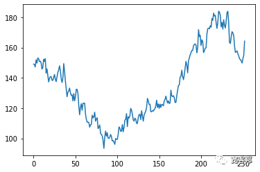
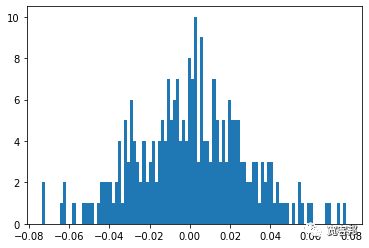
上面的代码基本上运行了一个交易年度(252 天)内潜在价格序列演变的单一模拟,基于遵循正态分布的每日收益随机的抽取。由第一个图表中显示的单线系列表示。第二个图表绘制了一年期间这些随机每日收益的直方图。
现在我们已经成功模拟了未来一年的每日价格数据。但实际上它并没有让我们深入了解股票的风险和回报特征,因为我们只有一个随机生成的路径。实际价格完全按照上表所述演变的可能性几乎为零。
那么你可能会问这个模拟有什么意义呢?好吧,真正的洞察力是通过运行数千次、数万次甚至数十万次模拟获得的,每次运行都会根据相同的股票特征(mu 和 vol)产生一系列不同的潜在价格演变。
我们可以非常简单地调整上面的代码来运行多个模拟。此代码如下所示。在下面的代码中,您会注意到一些事情——首先我删除了直方图(我们稍后会以稍微不同的方式回到这个问题),并且代码现在在一个图表上绘制多个价格系列以显示信息对于每个单独的模拟运行。
import numpy as npimport mathimport matplotlib.pyplot as pltfrom scipy.stats import norm
#Define VariablesS = apple['Adj Close'][-1] #starting stock price (i.e. last available real stock price)T = 252 #Number of trading daysmu = 0.2309 #Returnvol = 0.4259 #Volatility
#choose number of runs to simulate - I have chosen 1000for i in range(1000): #create list of daily returns using random normal distribution daily_returns=np.random.normal(mu/T,vol/math.sqrt(T),T)+1
#set starting price and create price series generated by above random daily returns
price_list = [S]
for x in daily_returns: price_list.append(price_list[-1]*x)
#plot data from each individual run which we will plot at the end plt.plot(price_list)
#show the plot of multiple price series created aboveplt.show()
这为我们提供了以下 1000 个不同模拟价格系列的图:
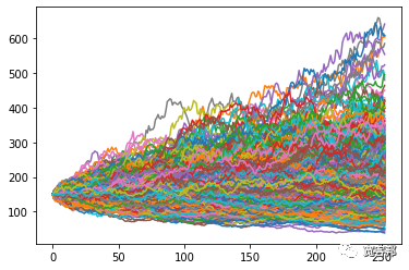
现在我们可以看到 1000 次不同模拟产生的潜在结果,考虑到每日收益序列的随机性,所有模拟都基于相同的基本输入。
最终价格的差价相当大,从大约 45 美元到 500 美元不等!
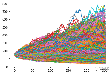
在当前的格式中,由于图表中充满了数据,因此很难真正清楚地看到正在发生的事情——所以这就是我们回到之前删除的直方图的地方,尽管这次它会向我们展示 结束模拟值的分布,而不是单个模拟的每日收益分布。这次我还模拟了 10,000 次运行,以便为我们提供更多数据。
同样,代码很容易调整以包含此直方图。
import numpy as npimport mathimport matplotlib.pyplot as pltfrom scipy.stats import norm
#set up empty list to hold our ending values for each simulated price seriesresult = []
#Define VariablesS = apple['Adj Close'][-1] #starting stock price (i.e. last available real stock price)T = 252 #Number of trading daysmu = 0.2309 #Return
vol = 0.4259 #Volatility
#choose number of runs to simulate - I have chosen 10,000for i in range(10000): #create list of daily returns using random normal distribution daily_returns=np.random.normal(mu/T,vol/math.sqrt(T),T)+1
#set starting price and create price series generated by above random daily returns price_list = [S]
for x in daily_returns: price_list.append(price_list[-1]*x)
#plot data from each individual run which we will plot at the end plt.plot(price_list)
#append the ending value of each simulated run to the empty list we created at the beginning result.append(price_list[-1])
#show the plot of multiple price series created aboveplt.show()
#create histogram of ending stock values for our mutliple simulationsplt.hist(result,bins=50)plt.show()
输出如下:
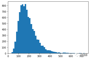
我们现在可以快速计算分布的平均值以获得我们的“预期值”:
#use numpy mean function to calculate the mean of the result
print(round(np.mean(result),2))
输出188.41。当然,您会得到略有不同的结果,因为这些是随机每日回报抽取的模拟。您在每次模拟中包含的路径或运行次数越多,平均值就越倾向于我们用作“mu”输入的平均回报。这是大数定律的结果。
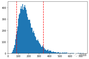
我们还可以查看潜在价格分布的几个“分位数”,以了解非常高或非常低回报的可能性。
我们可以使用 numpy 的“percentile”函数来计算 5% 和 95% 的分位数:
print("5% quantile =",np.percentile(result,5))print("95% quantile =",np.percentile(result,95))
5% quantile = 85.0268905204829495% quantile = 344.5558966477557
我们现在知道,股价有 5% 的可能性最终会低于 85.02 美元,有 5% 的可能性会高于 344.55 美元。
我们可以开始问自己这样的问题:“我是否愿意冒 5% 的风险最终获得价值低于 63.52 美元的股票,以追逐股价在 188.41 美元左右的预期回报?”
最后要做的就是在直方图上快速绘制我们刚刚计算的两个分位数,以给我们一个直观的表示。扫描本文最下方二维码获取全部完整源码和Jupyter Notebook 文件打包下载。
plt.hist(result,bins=100)plt.axvline(np.percentile(result,5), color='r', linestyle='dashed', linewidth=2)plt.axvline(np.percentile(result,95), color='r', linestyle='dashed', linewidth=2)plt.show()
↓↓长按扫码获取完整源码↓↓