
当价格和您的指标向相反方向移动时,就会出现背离。例如,您使用 RSI 进行交易,它上次在 80 处达到峰值,现在在 70 处达到峰值。当 RSI 达到 80 时,您交易的标的证券价格为 14 美元,现在达到新的峰值 18 美元。这是一个背离。
由于峰值的趋势,交易者将价格称为“更高的高点”,将 RSI 称为“更低的高点”。技术交易者通过视觉跟踪但很难复制,因为并不总是清楚究竟是什么造就了“峰值”。我们提供了一种算法来检测交易的波峰和波谷,我们将在下面深入探讨构建 RSI 背离策略的细节时加以利用。
作为入场信号的背离
背离通常被称为“看跌”或“看涨”。看跌背离就像我们在上面的例子中看到的那样。我们有一个动量指标在价格之前减弱,这给了我们一个做空的点。看涨背离是我们的动量指标出现较高的低点,但价格较低的低点。
根据这种解释,背离是领先指标——背离发生在价格行为确认之前。在实践中,实现这一点更具挑战性,因为您会发现自己正在寻找价格和指标的峰值,并且直到经过一段时间后才能确认该值是峰值,因此您可以查看该值是否下降。
无论如何,让我们用一些代码来说明这是如何工作的!
检测背离
第一步将需要导入几个包。
import numpy as npimport pandas as pdimport matplotlib.pyplot as pltimport yfinance as yffrom scipy.signal import argrelextremafrom collections import deque
argrelextrema 用于检测 SciPy 信号处理库中的峰值,而 deque 就像一个固定长度的列表,如果超过它的长度,它将删除最旧的条目并保留新条目。我们将使用第一个来发现数据中的极值,然后循环遍历它们并保留高于先前条目的点。
为了找出极值,我们需要传递一个名为 order 的参数。这定义了我们实际需要在峰的两侧有多少个点来标记峰。因此,当 order=5 时,我们需要一些东西成为左右 5 个数据点内的最高点。我们提供的另一个参数是 K,它只是一个整数,用于确定我们想要识别多少个连续峰值以确定更高的高点趋势。
下面给出了完整的、更高的检测功能。
def getHigherHighs(data: np.array, order=5, K=2): ''' Finds consecutive higher highs in price pattern. Must not be exceeded within the number of periods indicated by the width
parameter for the value to be confirmed. K determines how many consecutive highs need to be higher. ''' # Get highs high_idx = argrelextrema(data, np.greater, order=order)[0] highs = data[high_idx] # Ensure consecutive highs are higher than previous highs extrema = [] ex_deque = deque(maxlen=K) for i, idx in enumerate(high_idx): if i == 0: ex_deque.append(idx) continue if highs[i] < highs[i-1]: ex_deque.clear()
ex_deque.append(idx) if len(ex_deque) == K: extrema.append(ex_deque.copy())
return extrema
这将返回包含峰值索引的双端队列列表。为了获得用于识别背离的所有相关组合,我们需要四个这样的函数,一个用于更高的高点(上图)、更低的低点、更低的高点和更高的低点。它们中的每一个的逻辑都是相同的,我们只是在第 9 行将 np.greater 更改为 np.less 并在第 18 行更改不等号以获得我们想要的行为。
我们需要一些数据,因此我们将从 Yahoo! 使用 yfinance 包的金融 API。我将使用埃克森美孚 (XOM),因为它在过去几十年中经历了相当多的繁荣和萧条。
start = '2011-01-01'end = '2011-07-31'
ticker = 'XOM'yfObj = yf.Ticker(ticker)data = yfObj.history(start=start, end=end)
# Drop unused columnsdata.drop(['Open', 'High', 'Low', 'Volume', 'Dividends', 'Stock Splits'], axis=1, inplace=True)
现在我们可以计算所有的极值并绘制结果。
from matplotlib.lines import Line2D # For legend
price = data['Close'].valuesdates = data.index
# Get higher highs, lower lows, etc.order = 5hh = getHigherHighs(price, order)lh = getLowerHighs(price, order)ll = getLowerLows(price, order)hl = getHigherLows(price, order)
# Get confirmation indiceshh_idx = np.array([i[1] + order for i in hh])lh_idx = np.array([i[1] + order for i in lh])ll_idx = np.array([i[1] + order for i in ll])hl_idx = np.array([i[1] + order for i in hl])
# Plot resultscolors = plt.rcParams['axes.prop_cycle'].by_key()['color']
plt.figure(figsize=(12, 8))
plt.plot(data['Close'])plt.scatter(dates[hh_idx], price[hh_idx-order], marker='^', c=colors[1])plt.scatter(dates[lh_idx], price[lh_idx-order], marker='v', c=colors[2])plt.scatter(dates[ll_idx], price[ll_idx-order], marker='v', c=colors[3])plt.scatter(dates[hl_idx], price[hl_idx-order], marker='^', c=colors[4])_ = [plt.plot(dates[i], price[i], c=colors[1]) for i in hh]_ = [plt.plot(dates[i], price[i], c=colors[2]) for i in lh]_ = [plt.plot(dates[i], price[i], c=colors[3]) for i in ll]_ = [plt.plot(dates[i], price[i], c=colors[4]) for i in hl]
plt.xlabel('Date')plt.ylabel('Price ($)')plt.title(f'Potential Divergence Points for {ticker} Closing Price')legend_elements = [ Line2D([0], [0], color=colors[0], label='Close'), Line2D([0], [0], color=colors[1], label='Higher Highs'), Line2D([0], [0], color='w', marker='^', markersize=10, markerfacecolor=colors[1], label='Higher High Confirmation'), Line2D([0], [0], color=colors[2], label='Higher Lows'),
Line2D([0], [0], color='w', marker='^', markersize=10, markerfacecolor=colors[2], label='Higher Lows Confirmation'), Line2D([0], [0], color=colors[3], label='Lower Lows'), Line2D([0], [0], color='w', marker='v', markersize=10, markerfacecolor=colors[3], label='Lower Lows Confirmation'), Line2D([0], [0], color=colors[4], label='Lower Highs'), Line2D([0], [0], color='w', marker='^', markersize=10, markerfacecolor=colors[4], label='Lower Highs Confirmation')]plt.legend(handles=legend_elements, bbox_to_anchor=(1, 0.65))plt.show()
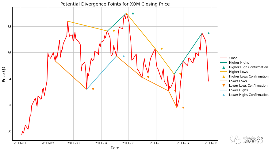
在这个图中,我们提取了所有潜在的分歧点,并将高点和低点映射到价格。另外,请注意我为每个峰值绘制了确认点。我们不知道峰值是否真的是峰值,直到我们给它几天(在这种情况下为 5 天)看看价格接下来会发生什么。
价格图表只是背离所需的一半,我们还需要应用一个指标。借鉴考夫曼出色的交易系统和方法,我们应该使用某种动量指标。我们将继续应用 RSI,尽管 MACD、随机指标等也适用。
RSI 的峰值和谷值
RSI 最常被解释为当该值高于中心线 (RSI=50) 时表现出上升势头,而当它低于中心线时表现出下降势头。如果我们有一系列高于 50 的较小峰值,则可能表明动能减弱,而低于 50 的一系列不断增加的谷可能表明我们可以交易的动能增加。
我们的下一步是计算 RSI,然后应用与上述相同的技术来提取相关的极值。
def calcRSI(data, P=14): data['diff_close'] = data['Close'] - data['Close'].shift(1) data['gain'] = np.where(data['diff_close']>0, data['diff_close'], 0) data['loss'] = np.where(data['diff_close']<0, np.abs(data['diff_close']), 0) data[['init_avg_gain', 'init_avg_loss']] = data[ ['gain', 'loss']].rolling(P).mean() avg_gain = np.zeros(len(data)) avg_loss = np.zeros(len(data)) for i, _row in enumerate(data.iterrows()): row = _row[1] if i < P - 1: last_row = row.copy() continue elif i == P-1: avg_gain[i] += row['init_avg_gain'] avg_loss[i] += row['init_avg_loss'] else: avg_gain[i] += ((P - 1) * avg_gain[i-1] + row['gain']) / P avg_loss[i] += ((P - 1) * avg_loss[i-1] + row['loss']) / P
last_row = row.copy()
data['avg_gain'] = avg_gain data['avg_loss'] = avg_loss
data['RS'] = data['avg_gain'] / data['avg_loss'] data['RSI'] = 100 - 100 / (1 + data['RS']) return data
有了该功能,我们可以将 RSI 及其相关列添加到我们的数据框中:
data = calcRSI(data.copy())# Get values to mark RSI highs/lows and plotrsi_hh = getHigherHighs(rsi, order)rsi_lh = getLowerHighs(rsi, order)rsi_ll = getLowerLows(rsi, order)rsi_hl = getHigherLows(rsi, order)
我们将遵循与上述相同的格式来绘制我们的结果:
fig, ax = plt.subplots(2, figsize=(20, 12), sharex=True)ax[0].plot(data['Close'])ax[0].scatter(dates[hh_idx], price[hh_idx-order], marker='^', c=colors[1])ax[0].scatter(dates[lh_idx], price[lh_idx-order], marker='v', c=colors[2])ax[0].scatter(dates[hl_idx], price[hl_idx-order], marker='^', c=colors[3])ax[0].scatter(dates[ll_idx], price[ll_idx-order], marker='v', c=colors[4])_ = [ax[0].plot(dates[i], price[i], c=colors[1]) for i in hh]_ = [ax[0].plot(dates[i], price[i], c=colors[2]) for i in lh]
_ = [ax[0].plot(dates[i], price[i], c=colors[3]) for i in hl]_ = [ax[0].plot(dates[i], price[i], c=colors[4]) for i in ll]
ax[0].set_ylabel('Price ($)')ax[0].set_title(f'Price and Potential Divergence Points for {ticker}')ax[0].legend(handles=legend_elements)
ax[1].plot(data['RSI'])ax[1].scatter(dates[rsi_hh_idx], rsi[rsi_hh_idx-order], marker='^', c=colors[1])ax[1].scatter(dates[rsi_lh_idx], rsi[rsi_lh_idx-order], marker='v', c=colors[2])ax[1].scatter(dates[rsi_hl_idx], rsi[rsi_hl_idx-order], marker='^', c=colors[3])ax[1].scatter(dates[rsi_ll_idx], rsi[rsi_ll_idx-order], marker='v', c=colors[4])_ = [ax[1].plot(dates[i], rsi[i], c=colors[1]) for i in rsi_hh]_ = [ax[1].plot(dates[i], rsi[i], c=colors[2]) for i in rsi_lh]_ = [ax[1].plot(dates[i], rsi[i], c=colors[3]) for i in rsi_hl]_ = [ax[1].plot(dates[i], rsi[i], c=colors[4]) for i in rsi_ll]
ax[1].set_ylabel('RSI')ax[1].set_title(f
'RSI and Potential Divergence Points for {ticker}')ax[1].set_xlabel('Date')
plt.tight_layout()plt.show()
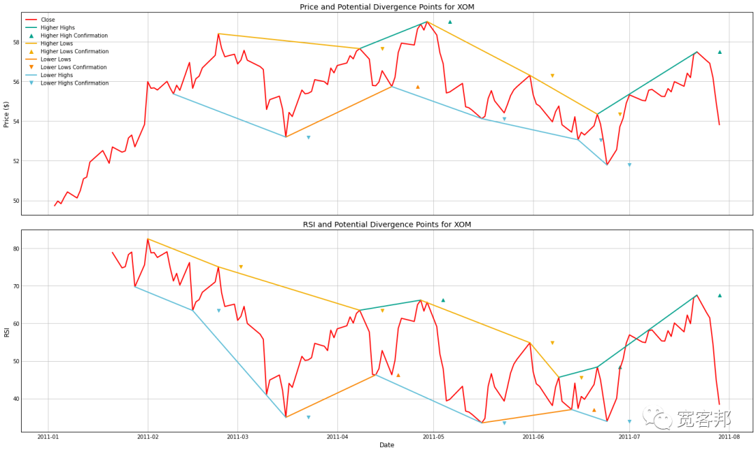
这只是一个短暂的 7 个月窗口,因此我们可以清楚地看到价格和 RSI 的走势,因此只有一个背离可见。我们在 RSI 图表(橙色,向上的三角形)上看到 6 月中旬在价格图表(蓝色,向下的三角形)中一系列较低的低点中间确认更高的低点。我们不权衡图表,所以让我们把一个算法放在一起来测试这个 RSI 背离模型。
建立 RSI 发散模型
到目前为止,我们有一些通用规则来识别我们有背离的情况,但我们仍然需要进入和退出规则。首先,我们可以求助于 Kaufmann 出色的交易系统和方法,在那里他列出了一个示例策略,其中包含以下规则:
如果指标高于目标水平(例如 RSI = 50),则在确定背离时输入头寸。如果指标背离消失,则退出。如果我们在价格创出更高的高点而 RSI 创出更低的高点时做空,那么我们的 RSI 会移动到更高的高点,那么我们就出局了。一旦指标达到目标水平就退出。允许背离转换为趋势位置。为此,我们使用单独的趋势指标(例如 EMA 交叉),如果趋势与背离方向相同,我们将持有头寸。如果背离消失但趋势继续,我们持有,并仅在趋势消失时退出。我们将根据 Kaufmann 规则构建两种模型,一种仅交易背离(规则 1-3),另一种具有背离加趋势(所有 4 条规则)。当然,您可以根据自己的需要随意修改这些,并自己尝试各种方法。
接下来,我将构建一些辅助函数来标记我们的峰值。第一组将修改我们的 getHigherHighs 函数组的输出。这些是为上述可视化而构建的,但我们只需要为我们的模型提取趋势的确认点。另请注意,由于我们正在向索引添加顺序,因此我们可能会获得会引发索引错误的确认点,因此我们会删除任何大于我们拥有的数据点数量的索引。
四个函数如下:
def getHHIndex(data: np.array, order=5, K=2): extrema = getHigherHighs(data, order, K) idx = np.array([i[-1] + order for i in extrema]) return idx[np.where(idx
def getLHIndex(data: np.array, order=5, K=2): extrema = getLowerHighs(data, order, K) idx = np.array([i[-1] + order for i in extrema]) return idx[np.where(idx
def getLLIndex(data: np.array, order=5, K=2): extrema = getLowerLows(data, order, K) idx = np.array([i[-1] + order for i in extrema])
return idx[np.where(idx
def getHLIndex(data: np.array, order=5, K=2): extrema = getHigherLows(data, order, K) idx = np.array([i[-1] + order for i in extrema]) return idx[np.where(idx
为了减少重写代码,我将引入一个名为 getPeaks 的函数,它获取我们的数据帧并将我们的高点和低点的输出编码为列向量。它将使用我们上面定义的四个函数,并从我们触及更高高点到 Close_highs 列分配值 1。如果我们的高点在确认较低的高点后呈下降趋势,那么我们在同一列中用 -1 标记。它会为低点做同样的事情。记住哪些值为 1 哪些值为 -1 很重要,因此如果趋势正在增加(更高的高点或更高的低点),我将其设为 1,如果趋势正在下降(更低的高点或更低的低点),我将其设为 1 )。
def getPeaks(data, key='Close', order=5, K=2):  vals = data[key].values  hh_idx = getHHIndex(vals, order, K)  lh_idx = getLHIndex(vals, order, K)  ll_idx = getLLIndex(vals, order, K)  hl_idx = getHLIndex(vals, order, K)
  data[f'{key}_highs'] = np.nan  data[f'{key}_highs'][hh_idx] = 1  data[f'{key}_highs'][lh_idx] = -1  data[f'{key}_highs'] = data[f'{key}_highs'].ffill().fillna(0)  data[f'{key}_lows'] = np.nan  data[f'{key}_lows'][ll_idx] = 1  data[f'{key}_lows'][hl_idx] = -1  data[f'{key}_lows'] = data[f'{key}_highs'].ffill().fillna(0)  return data
最后,我们可以制定我们的战略。在这里,我们只是遵循上面列出的前 3 条规则。
def RSIDivergenceStrategy(data, P=14, order=5, K=2): ''' Go long/short on price and RSI divergence. - Long if price to lower low and RSI to higher low with RSI < 50 - Short if price to higher high and RSI to lower high with RSI > 50 Sell if divergence disappears. Sell if the RSI crosses the centerline. ''' data = getPeaks(data, key='Close', order=order, K=K) data = calcRSI(data, P=P) data = getPeaks(data, key='RSI', order=order, K=K)
position = np.zeros(data.shape[0]) # position[:] = np.nan for i, (t, row) in enumerate(data.iterrows()): if np.isnan(row['RSI']): continue # If no position is on if position[i-1] == 0: # Buy if indicator to higher low and price to lower low if row['Close_lows'] == -1 and row['RSI_lows'] == 1:
if row['RSI'] < 50: position[i] = 1 entry_rsi = row['RSI'].copy()
# Short if price to higher high and indicator to lower high elif row['Close_highs'] == 1 and row['RSI_highs'] == -1: if row['RSI'] > 50: position[i] = -1 entry_rsi = row['RSI'].copy()
# If current position is long elif position[i-1] == 1: if row['RSI'] < 50 and row['RSI'] < entry_rsi: position[i] = 1
# If current position is short elif position[i-1] == -1: if row['RSI'] < 50 and row['RSI'] > entry_rsi: position[i] = -1
data['position'] = position return calcReturns(data)
def calcReturns(df): # Helper function to avoid repeating too much code
df['returns'] = df['Close'] / df['Close'].shift(1) df['log_returns'] = np.log(df['returns']) df['strat_returns'] = df['position'].shift(1) * df['returns'] df['strat_log_returns'] = df['position'].shift(1) * df['log_returns'] df['cum_returns'] = np.exp(df['log_returns'].cumsum()) - 1 df['strat_cum_returns'] = np.exp(df['strat_log_returns'].cumsum()) - 1 df['peak'] = df['cum_returns'].cummax() df['strat_peak'] = df['strat_cum_returns'].cummax() return df
关于退出条件需要注意的一件事,我们要等待趋势的变化。我没有等待 5 天来确认 RSI 的峰值,而是添加了一个条件,即如果 RSI 跌破我们的多头仓位的入场 RSI 或高于我们的空头仓位的入场 RSI,我们应该退出。这是有效的,因为如果我们在 RSI 的较低高点做空,那么如果情况逆转,我们将退出。如果 RSI 收于我们的入场 RSI 上方,那么要么成为更高的高点,从而打破我们的趋势,要么更高的高点仍将到来。设置这个条件只会让我们更快地退出交易。
好了,解释够了,让我们用 2000-2020 年的数据测试一下。
start = '2000-01-01'end = '2020-12-31'data = yfObj.history(start=start, end=end)# Drop unused columnsdata.drop(['Open', 'High', 'Low', 'Volume', 'Dividends', 'Stock Splits'], axis=1, inplace=True)
df_div = RSIDivergenceStrategy(data.copy())
plt.figure(figsize=(12, 8))plt.plot(df_div['cum_returns'] * 100, label='Buy-and-Hold')
plt.plot(df_div['strat_cum_returns'] * 100, label='RSI Divergence')plt.xlabel('Date')plt.ylabel('Returns (%)')plt.title(f'Buy-and-Hold and RSI Divergence Returns for {ticker}')plt.legend()plt.show()
df_stats = pd.DataFrame(getStratStats(df_div['log_returns']), index=['Buy and Hold'])df_stats = pd.concat([df_stats, pd.DataFrame(getStratStats(df_div['strat_log_returns']), index=['Divergence'])])
df_stats
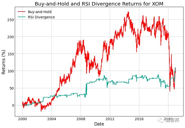

最后,背离策略的表现优于买入并持有的策略(忽略埃克森美孚支付的股息)。它的波动性较小,跌幅较小,但在 2004 年至 2020 年期间表现不佳。换句话说,在 2020 年突破之前,你会等待 16 年,而这种策略看起来像是对底层证券的亏损。这种策略可能在其他地方更有效或适合多元化的投资组合,但至少在这种情况下, 纯 RSI 背离策略看起来不太好。
RSI 背离和趋势
对于下一个模型,让我们采用 Kaufman 的建议并应用趋势转换。为此,我们将选择 EMA 交叉。因此,该模型将像我们上面看到的背离模型一样进行交易,但会检查我们的 EMA 交叉所指示的趋势。如果我们做多且 EMA1 > EMA2,我们将保持该头寸。
EMA 计算代码和策略如下:
def _calcEMA(P, last_ema, N): return (P - last_ema) * (2 / (N + 1)) + last_ema
def calcEMA(data, N): # Initialize series data['SMA_' + str(N)] = data['Close'].rolling(N).mean()
ema = np.zeros(len(data)) for i, _row in enumerate(data.iterrows()): row = _row[1] if i < N: ema[i] += row['SMA_' + str(N)] else: ema[i] += _calcEMA(row['Close'], ema[i-1], N) data['EMA_' + str(N)] = ema.copy() return data
def RSIDivergenceWithTrendStrategy(data, P=14, order=5, K=2, EMA1=50, EMA2=200): ''' Go long/short on price and RSI divergence. - Long if price to lower low and RSI to higher low with RSI < 50 - Short if price to higher high and RSI to lower high with RSI > 50 Sell if divergence disappears or if the RSI crosses the centerline, unless there is a trend in the same direction. ''' data = getPeaks(data, key='Close', order=order, K=K) data = calcRSI(data, P=P) data = getPeaks(data, key='RSI', order=order, K=K) data = calcEMA(data, EMA1) data = calcEMA(data, EMA2)
position = np.zeros(data.shape[0]) # position[:] = np.nan for i, (t, row) in enumerate(data.iterrows()): if np.isnan(row['RSI']): continue # If no position is on if position[i-1] == 0: # Buy if indicator to higher high and price to lower high if row['Close_lows'] == -1 and row['RSI_lows'] == 1: if row['RSI'] < 50: position[i] = 1 entry_rsi = row['RSI'].copy()
# Short if price to higher high and indicator to lower high elif row['Close_highs'] == 1 and row['RSI_highs'] == -1: if row['RSI'] > 50: position[i] = -1 entry_rsi = row['RSI'].copy()
# If current position is long elif position[i-1] == 1: if row['RSI'] < 50 and row['RSI'] < entry_rsi: position[i] = 1
elif row[f'EMA_{EMA1}'] > row[f'EMA_{EMA2}']: position[i] = 1
# If current position is short elif position[i-1] == -1: if row['RSI'] < 50 and row['RSI'] > entry_rsi: position[i] = -1 elif row[f'EMA_{EMA1}'] < row[f'EMA_{EMA2}']: position[i] = -1
data['position'] = position return calcReturns(data)
在我们的数据上运行这个模型,我们得到:
plt.figure(figsize=(12, 8))plt.plot(df_trend['cum_returns'] * 100, label=f'Buy-and-Hold')plt.plot(df_trend['strat_cum_returns'] * 100, label='RSI Div + Trend')plt.xlabel('Date')plt.ylabel('Returns (%)')plt.title(f'Buy-and-Hold and Divergence with Trend Returns for {ticker}')plt.legend()plt.show()
df_trend = RSIDivergenceWithTrendStrategy(data.copy())df_stats = pd.concat([df_stats, pd.DataFrame(getStratStats(df_trend['strat_log_returns']),
index=['Div + Trend'])])df_stats
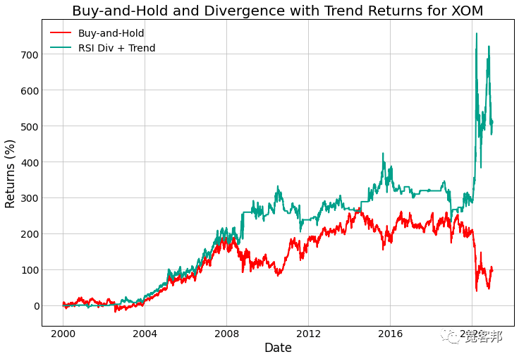
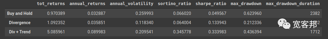
添加我们的趋势指标大大增加了我们的回报。它以较低的波动性(尽管比 RSI 背离策略更多)和较高的风险调整回报。最大回撤小于底层证券经历的最大回撤,而且持续时间更短。
你准备好交易了吗?
我们研究了两种 RSI 背离策略的编码和交易,一种很好,另一种则不然。这是否意味着您应该出去用 EMA 交叉交易 RSI 背离?
在这里给你一些关于这些指标的想法和解释。这些快速的回测很有用,因为您可以了解如何测试想法,并且可以在各种证券和市场上进行测试以开始缩小选择范围。也许更严格的测试表明 RSI 背离是您系统中真正有价值的部分,而趋势模型是一个异常值。除非你测试它,否则你永远不会知道!
扫描本文最下方二维码获取全部完整源码和Jupyter Notebook 文件打包下载。