
布林带(BOLL)指标是美国股市分析家约翰·布林根据统计学中的标准差原理设计出来的一种非常简单实用的技术分析指标。一般而言,股价的运动总是围绕某一价值中枢(如均线、成本线等)在一定的范围内变动,布林线指标正是在上述条件的基础上,引进了“股价通道”的概念,其认为股价通道的宽窄随着股价波动幅度的大小而变化,而且股价通道又具有变异性,它会随着股价的变化而自动调整。
我们可以根据它来开发许多不同的算法策略进行测试。下面,我们将介绍 4 种不同的交易策略,这些策略依赖于均值回归和趋势跟踪的波段。
布林带和均值回归
对于标准布林带设置,我们查看典型价格的 20 天移动平均线。如果典型价格遵循正态分布,则它有大约 5% 的机会将 2 个或更多标准差从均值移开。换句话说,我们有 1/20 的机会到达标准布林带的边缘。
均值回归交易者看到这一点,并希望押注价格将在短期内回到 SMA(TP)。因此,如果我们触及上布林带 (UBB),我们就会做空,如果我们触及下布林带 (LBB),我们就会做多并持有,直到我们到达 SMA(TP)。
下面我们将开始编写此策略并查看其执行情况。让我们导入一些基本的包。
import numpy as npimport pandas as pdimport matplotlib.pyplot as pltimport yfinance as yf
接下来我将编写一个函数来计算我们的布林带。
def calcBollingerBand(data, periods=20, m=2, label=None): '''Calculates Bollinger Bands''' keys = ['UBB', 'LBB', 'TP', 'STD', 'TP_SMA'] if label is None: ubb, lbb, tp, std, tp_sma = keys else: ubb, lbb, tp, std, tp_sma = [i + '_' + label for i in keys] data[tp] = data.apply( lambda x: np.mean(x[['High', 'Low', 'Close']]), axis=1) data[tp_sma] = data[tp].rolling(periods) data[std] = data[tp].rolling(periods) data[ubb] = data[tp_sma] + m * data[std] data[lbb] = data[tp_sma] - m * data[std] return data
这将从 YFinance 雅虎财经 获取我们需要的数据并计算所有必要的中间值,然后输出典型价格 (TP)、SMA(TP) (TP_SMA)、上布林带 (UBB) 和下布林带 (LBB)。除了我们的数据之外,它还需要我们在计算中使用的周期数(periods)和标准差数 (m)。我还添加了一个可选的标签参数,它将更新数据中的键,因为我们将研究的某些策略使用两组布林带,并且我们不希望在进行计算时覆盖这些值。
接下来,我们将编写均值回归策略。
def BBMeanReversion(data, periods=20, m=2, shorts=True): ''' Buy/short when price moves outside of bands. Exit position when price crosses SMA(TP). ''' data = calcBollingerBand(
data, periods) xs = (data['Close'] - data['TP_SMA']) / \ (data['Close'].shift(1) - data['TP_SMA'].shift(1))
data['position'] = np.nan data['position'] = np.where(data['Close']<=data['LBB'], 1, data['position']) if shorts: data['position'] = np.where(data['Close']>=data['UBB'], -1, data['position']) else: data['position'] = np.where(data['Close']>=data['UBB'], 0, data['position'])
data['position'] = np.where(np.sign(xs)==-1, 0, data['position'])
data['position'] = data['position'].ffill() return calcReturns(data)
当价格移动到 LBB 时,该策略将做多,当价格到达 UBB 时做空。如果价格穿过 SMA(TP),它将卖出。我们通过寻找收盘价和 SMA(TP) 之间的差异从一天到下一天的迹象变化来做到这一点。
最后,你会看到我们不是简单地返回数据,而是将它包装在一个 calcReturns函数中。这是一个辅助函数,可以轻松获得我们的策略和买入并持有基准的回报,我们将以此为基准进行回测。
def calcReturns(df): # Helper function to avoid repeating too much code df['returns'] = df['Close'] / df['Close'].shift(1) df['log_returns'] = np.log(df['returns']) df['strat_returns'] = df['position'].shift(1) * df['returns'] df['strat_log_returns'] = df['position'].shift(1) * \ df['log_returns'] df['cum_returns'] = np.exp(df['log_returns']) - 1 df['strat_cum_returns'] = np.exp(df['strat_log_returns'].cumsum()) - 1 df['peak'] = df['cum_returns'].cummax() df['strat_peak'] = df['strat_cum_returns'].cummax() return df
现在只需要输入我们的数据,就可以看看这个策略是如何执行的。我将只从标准普尔 500 指数中获取一些数据,并在 2000 年至 2020 年的 21 年间对其进行测试。
table = pd.read_html('https://en.wikipedia.org/wiki/List_of_S%26P_500_companies')df = table[0]syms = df['Symbol']ticker = np.random.choice(syms.values)print(f"Ticker Symbol: {ticker}")
start = '2000-01-01'end = '2020-12-31'
yfObj = yf.Ticker(ticker)data = yfObj.history(start=start, end=end)data.drop(['Open', 'Volume', 'Dividends', 'Stock Splits'], inplace=True, axis=1)
df_rev = BBMeanReversion(data.copy(), shorts=True)
colors = plt.rcParams['axes.prop_cycle']
fig, ax = plt.subplots(2, figsize=(15, 10), sharex=True)
ax[0].plot(df_rev['Close'], label='Close')ax[0].plot(df_rev['TP_SMA'], label='SMA(TP)')ax[0].plot(df_rev['UBB'], color=colors[2])ax[0].plot(df_rev['LBB'], color=colors[2])ax[0].fill_between(df_rev.index, df_rev['UBB'], df_rev['LBB'], alpha=0.3, color=colors[2], label='Bollinger Band')
ax[0].set_ylabel('Price ($)')ax[0].set_title(f'Price and Indicators for {ticker}')ax[0].legend()
ax[1].plot(df_rev['cum_returns']*100, label='Buy and Hold')ax[1].plot(df_rev['strat_cum_returns']*100, label='Mean Reversion')ax[1].set_xlabel('Date')ax[1].set_ylabel('Returns (%)')ax[1].set_title(f'Buy and Hold and Mean Reversion Returns for {ticker}')ax[1].legend()
plt.tight_layout()plt.show()
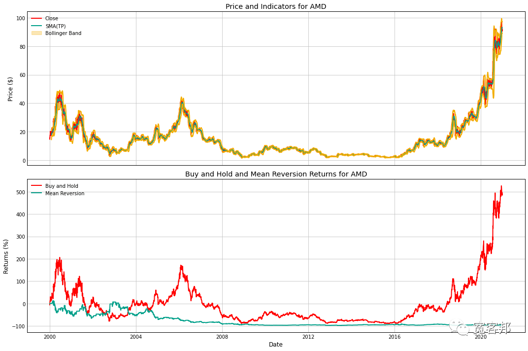
在21 年尺度上很容易看出这种策略与简单的买入并持有方法相比基本持平。
让我们使用另一个辅助函数来获取这两个的统计数据,以便我们可以更深入一些。
def getStratStats(log_returns: pd.Series, risk_free_rate: float = 0.02): stats = {}
# Total Returns stats['tot_returns'] = np.exp(log_returns.sum()) - 1
# Mean Annual Returns stats['annual_returns'] = np.exp(log_returns.mean() * 252) - 1
# Annual Volatility stats['annual_volatility'
] = log_returns.std() * np.sqrt(252)
# Sortino Ratio annualized_downside = log_returns.loc[log_returns].std() * \ np.sqrt(252) stats['sortino_ratio'] = (stats['annual_returns'] - \ risk_free_rate) / annualized_downside
# Sharpe Ratio stats['sharpe_ratio'] = (stats['annual_returns'] - \ risk_free_rate) / stats['annual_volatility']
# Max Drawdown cum_returns = log_returns.cumsum() peak = cum_returns.cummax() drawdown = peak - cum_returns stats['max_drawdown'] = drawdown.max()
# Max Drawdown Duration strat_dd = drawdown[drawdown==0] strat_dd_diff = strat_dd.index[1:] - strat_dd.index[:-1] strat_dd_days = strat_dd_diff.map(lambda x: x.days).values strat_dd_days = np.hstack([strat_dd_days, (drawdown.index[-1] - strat_dd.index[-1]).days]) stats['max_drawdown_duration'] = strat_dd_days.max() return stats
bh_stats = getStratStats(df_rev['log_returns'])rev_stats = getStratStats(df_rev['strat_log_returns'])
df = pd.DataFrame(bh_stats, index=['Buy and Hold'])df = pd.concat([df, pd.DataFrame(rev_stats, index=['Mean Reversion'])])df

总的来说,这个策略的效果很差,几乎损失了我们所有的本金。但情况并不总是如此,下面我们可以看到该策略与买入并持有方法的年化表现。
df_rev['year'] = df_rev.index.map(lambda x: x.year)ann_rets = df_rev.groupby('year')[['log_returns', 'strat_log_returns']].sum()ann_rets.columns = ['Buy and Hold Returns', 'Mean Reversion Returns']ann_rets.apply(lambda x: np.exp(x).round(4), axis=1)* 100
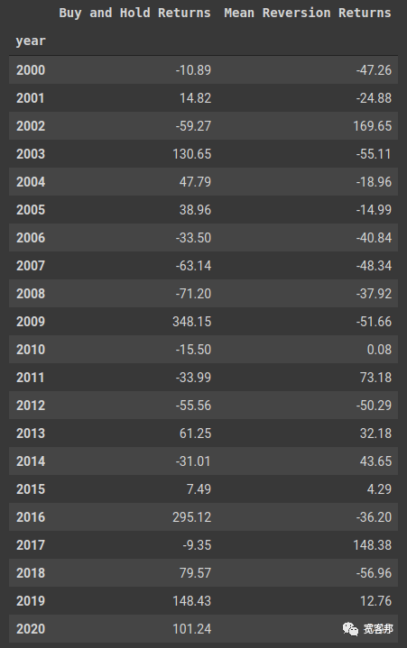
我们的均值回归模型要么非常厉害,要么非常差劲。从 2003 年到 2009 年,它只是年复一年地以可怕的速度增加损失,使其不可能再回来。此外,我们可以看到这只股票以及策略具有非常高的波动性——对于这些策略来说,这通常是一件好事——但它经常被误入歧途。
long_entry = df_rev.loc[(df_rev['position']==1) & (df_rev['position'].shift(1)==0)]['Close']
long_exit = df_rev.loc[(df_rev['position']==0) & (df_rev['position'].shift(1)==1)]['Close']short_entry = df_rev.loc[(df_rev['position']==-1) & (df_rev['position'].shift(1)==0)]['Close']short_exit = df_rev.loc[(df_rev['position']==0) & (df_rev['position'].shift(1)==-1)]['Close']
colors = plt.rcParams['axes.prop_cycle'].by_key()['color']
fig, ax = plt.subplots(1, figsize=(15, 10), sharex=True)
ax.plot(df_rev['Close'], label='Close')ax.plot(df_rev['TP_SMA'], label='SMA(TP)')ax.plot(df_rev['UBB'], color=colors[2])ax.plot(df_rev['LBB'], color=colors[2])ax.fill_between(df_rev, df_rev['UBB'], df_rev['LBB'], alpha=0.3, color=colors[2], label='Bollinger Band')
ax.scatter(long_entry.index, long_entry, c=colors[4], s=100, marker='^', label='Long Entry', zorder=10)ax.scatter(long_exit.index, long_exit, c=colors[4], s=100, marker='x', label='Long Exit', zorder=10)ax.scatter(short_entry.index, short_entry, c=colors[3], s=100, marker='^', label='Short Entry', zorder=10)ax.scatter(short_exit.index, short_exit, c=colors[3], s=100, marker='x', label
='Short Exit', zorder=10)ax.set_ylabel('Price ($)')ax.set_title( f'Price and Bollinger Band Mean Reversion Strategy for {ticker} in 2002')ax.legend()
ax.set_ylim([0, 20])ax.set_xlim([pd.to_datetime('2002-01-01'), pd.to_datetime('2002-12-31')])plt.tight_layout()plt.show()
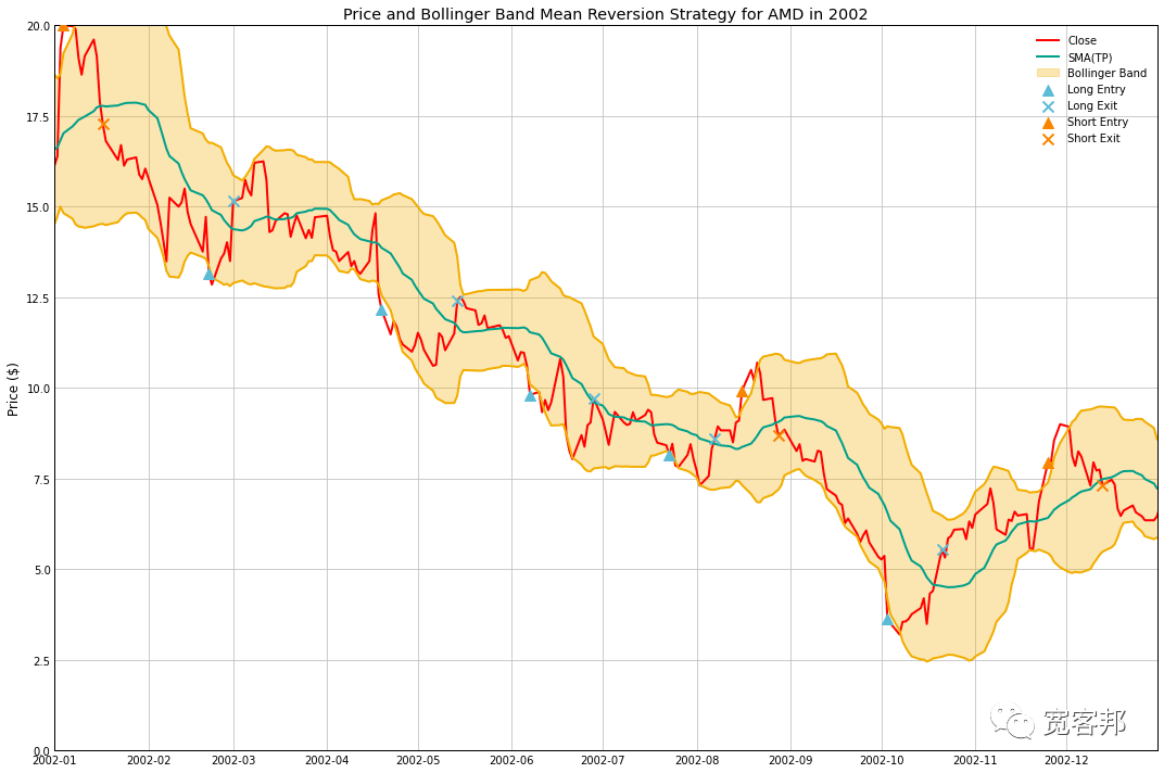
事实证明,2002 年的熊市标志是我们策略中为数不多的亮点之一。
布林带突破交易
均值回归表现不佳,但我们可以改用趋势跟踪模型,当价格移动到上频带上方时买入。
def BBBreakout(data, periods=20, m=1, shorts=True):  '''  Buy/short when price moves outside of the upper band.  Exit when the price moves into the band.  '''  data = calcBollingerBand(data, periods, m)
  data['position'] = np.nan  data['position'] = np.where(data['Close']>data['UBB'], 1, 0)  if shorts:    data['position'] = np.where(data['Close']<data['LBB'], -1, data['position'])  data['position'] = data['position'].ffill()
  return calcReturns(data)
df_break = BBBreakout(data.copy())
fig, ax = plt.subplots(2, figsize=(15, 10), sharex=True)
ax[0].plot(df_break['Close'], label='Close')
ax[0].plot(df_break['UBB'], color=colors[2])ax[0].plot(df_break['LBB'], color=colors[2])ax[0].fill_between(df_break.index, df_break['UBB'], df_break['LBB'], alpha=0.3, color=colors[2], label='Bollinger Band')ax[0].set_ylabel('Price ($)')ax[0].set_title(f'Price and Bolling Bands for {ticker}')ax[0].legend()
ax[1].plot(df_break['cum_returns'] * 100, label='Buy and Hold')ax[1].plot(df_break['strat_cum_returns'] * 100, label='Breakout')ax[1].set_xlabel('Date')ax[1].set_ylabel('Returns (%)')ax[1].set_title('Cumulative Returns for Breakout Strategy and Buy and Hold')ax[1].legend()
plt.show()
break_stats = getStratStats(df_break['strat_log_returns'])df = pd.concat([df, pd.DataFrame(break_stats, index=['Breakout'])])df
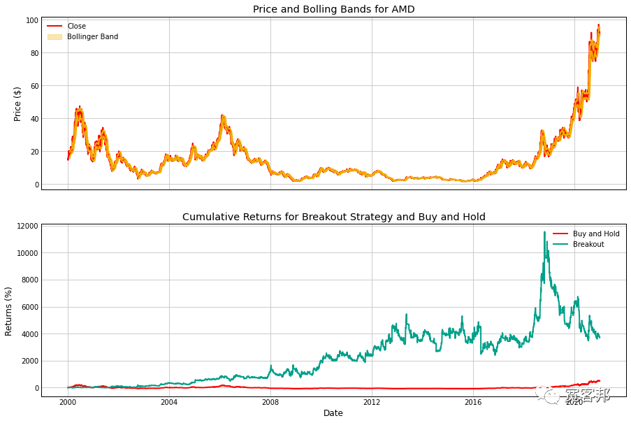
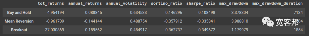
这个策略只是通过将起始资本乘以 37 倍来打破基线!夏普比 和 索提诺比率 的比率看起来也很合理。然而,最重要的是,该策略在 2018 年飙升并在随后的几年中几乎全部收回后出现了大幅回撤。
让我们仔细看看。
long_entry = df_break.loc[(df_break['position']==1) &                        (df_break['position'].shift(1)!=1)]['Close']long_exit = df_rev.loc[(df_break['position']!=1) &                        (df_break['position'].shift(1)==1)]['Close']short_entry = df_rev.loc[(df_break['position']==-1) &                        (df_break['position'].shift(1)!=-1)]['Close']short_exit = df_rev.loc[(df_break['position']!=-1) &                        (df_break['position'].shift(1)==-1)]['Close']
fig, ax = plt.subplots(figsize=(15, 10), sharex=True)
ax[0].plot(df_break['Close'], label='Close')ax[0].plot(df_break['UBB'], color=colors[2])ax[0].plot(df_break['LBB'], color=colors[2])ax[0].fill_between(df_break.index, df_break['UBB'], df_break['LBB'],                alpha=0.3, color=colors[2], label='Bollinger Band')ax[0].set_ylabel('Price ($)')ax[0].set_title(f'Price and Bolling Bands for {ticker} (2018)')ax[0].legend()
ax[0].scatter(long_entry.index, long_entry, c=colors[4],            s=100, marker='^', label='Long Entry',           zorder=10)ax[0].scatter(long_exit.index, long_exit, c=colors[4],           s=100, marker='x', label='Long Exit',           zorder=10)ax[0].scatter(short_entry.index, short_entry, c=colors[3],            s=100, marker='^', label='Short Entry',           zorder=10)ax[0].scatter(short_exit.index, short_exit, c=colors[3],           s=100, marker='x', label='Short Exit',           zorder=10)ax[0].set_ylim([5, 35])
ax[1].plot(df_break['strat_cum_returns'] * 100, label='Breakout', c=colors[1])ax[1].set_xlabel('Date')ax[1].set_ylabel('Returns (%)')ax[1].set_title('Cumulative Returns for Breakout Strategy')ax[1].legend()
ax[1].set_xlim([pd.to_datetime('2018-01-01'), pd.to_datetime('2019-01-01')])
plt.show()
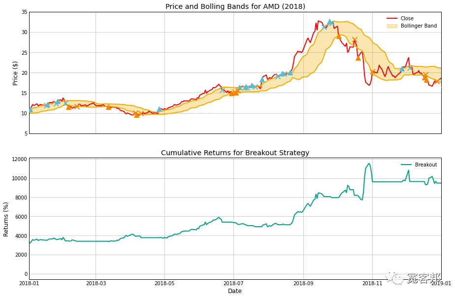
在上图中,我们看到 2018 年对于该模型来说几乎是完美的一年。当标的证券价格上涨 3 倍时,我们的模型几乎在每笔交易的右侧,并且能够从低点到高点将其净值增加 3 倍。它从 10 月下旬的峰值回落了一点,当时空头头寸逆向移动并带走了一点利润。
然后,发生了回撤。
fig, ax = plt.subplots(2, figsize=(15, 10), sharex=True)
ax[0].plot(df_break['Close'], label='Close')ax[0].plot(df_break['UBB'], color=colors[2])ax[0].plot(df_break['LBB'], color=colors[2])ax[0].fill_between(df_break.index, df_break['UBB'], df_break['LBB'],                alpha=0.3, color=colors[2], label='Bollinger Band')ax[0].set_ylabel('Price ($)')ax[0].set_title(f'Price and Bolling Bands for {ticker} (2019-2020)')ax[0].legend()
ax[0].scatter(long_entry.index, long_entry, c=colors[4],            s=100, marker='^', label='Long Entry',           zorder=10)ax[0].scatter(long_exit.index, long_exit, c=colors[4],           s=100, marker='x', label='Long Exit',           zorder=10)ax[0].scatter(short_entry.index, short_entry, c=colors[3],            s=100, marker='^', label='Short Entry',           zorder=10)ax[0].scatter(short_exit, short_exit, c=colors[3],           s=100, marker='x', label='Short Exit',           zorder=10)ax[0].set_ylim([15, 60])
ax[1].plot(df_break['strat_cum_returns'] * 100, label='Breakout', c=colors[1])ax[1].set_xlabel('Date')ax[1].set_ylabel('Returns (%)')ax[1].set_title('Cumulative Returns for Breakout Strategy')ax[1].legend()
ax[1].set_xlim([pd.to_datetime('2019-01-01'), pd.to_datetime('2020-06-01')])ax[1].set_ylim([3500, 10000])plt.show()
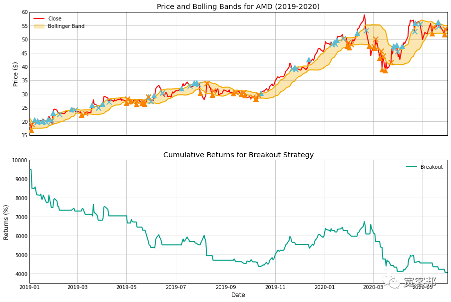
在 2019 年,我们的模型无法进行任何操作。它下跌了很多,因为它在年初的一系列虚假突破中不断亏损。大约在2020年年中,它发生了变化,一次又一次地向下行方向亏损。它在今年晚些时候出现了两次不错的上涨趋势,但这还不足以弥补迄今为止所遭受的损失。
当新冠疫情导致崩盘来临时,它一直被误入歧途,在大幅下跌之后卖空,结果却看到价格逆转,并被迫亏本平仓。
总体而言,该模型的性能非常出色。但是让我们看看我们是否可以通过添加另一个布林带,在价格反转之前移动得太远时进行卖出操作来做得更好。
双布林带突破
对于下一个策略,我们将在模型突破设定为 1σ 的内带时买入,但如果价格超出第二个带 2σ 则卖出。我们想要捕捉突破模型的优势,但在它们逆转我们之前进行平仓。
def DoubleBBBreakout(data, periods=20, m1=1, m2=2, shorts=True):  '''  Buy/short when price moves outside of the inner band (m1).  Exit when the price moves into the inner band or to the outer bound (m2).  '''  assert m2 > m1, f'm2 must be greater than m1:\nm1={m1}\tm2={m2}'  data = calcBollingerBand(data, m1, label='m1')  data = calcBollingerBand(data, m2, label='m2')
  data['position'] = np.nan  data['position'] = np.where(data['Close']>data['UBB_m1'], 1, 0)  if shorts:    data['position'] = np.where(data['Close']'LBB_m1'], -1, data['position'])  data['position'] = np.where(data['Close']>data['UBB_m2'], 0, data['position'])  data['position'] = np.where(data['Close']'LBB_m2'], 0, data['position'])  data['position'] = data['position'].ffill().fillna(0)
  return calcReturns(data)
df_double = DoubleBBBreakout(data.copy())
fig, ax = plt.subplots(2, figsize=(15, 10), sharex=True)
ax[0].plot(df_double['Close'], label='Close', linewidth=0.5)ax[0].plot(df_double['UBB_m1'], color=colors[2], linewidth=0.5)ax[0].plot(df_double['LBB_m1'], color=colors[2], linewidth=0.5)ax[0].fill_between(df_double.index, df_double['UBB_m1'], df_double['LBB_m1'], alpha=0.3, color=colors[2], label='Inner Bollinger Band')
ax[0].plot(df_double['UBB_m2'], color=colors[4], linewidth=0.5)ax[0].plot(df_double['LBB_m2'], color=colors[4], linewidth=0.5)ax[0].fill_between(df_double.index, df_double['UBB_m2'], df_double['LBB_m2'], alpha=0.3, color=colors[4], label='Outer Bollinger Band')ax[0].set_ylabel('Price ($)')ax[0].set_title(f'Price and Bolling Bands for {ticker}')ax[0].legend()
ax[1].plot(df_double['cum_returns'] * 100, label='Buy and Hold')ax[1].plot(df_double['strat_cum_returns'] * 100, label='Double Breakout')ax[1].set_xlabel('Date')ax[1].set_ylabel('Returns (%)')ax[1].set_title('Cumulative Returns for Double Breakout Strategy and Buy and Hold')ax[1].legend()
plt.show()
double_stats = getStratStats(df_double['strat_log_returns'])df = pd.concat([df, pd.DataFrame(double_stats, index=['Double Breakout'])])df
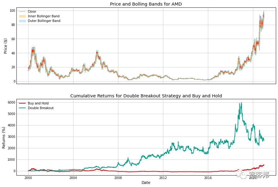
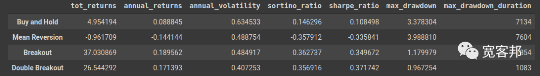
正如所希望的那样,与买入并持有以及之前的突破模型相比,该模型确实降低了我们的波动性。然而,我们的总回报有所下降 —— 仍然优于买入并持有模型和均值回归方法。令人惊讶的是,我们还降低了与突破模型相比的 Sortino 比率,但确实增加了我们的夏普比率。
交易带宽
John Bollinger 推荐的一种依赖于带宽的策略,是通过取 UBB 和 LBB 之间的差异并除以 SMA(TP) 来计算的。
随着宽度减小,波动性减小。Bollinger指出,当这种情况发生时,我们可以预期在带宽变低后波动性会增加。然而我们没有任何与低波动性相关的方向指标,所以我们需要将其与其他东西结合起来,让我们知道我们应该做多还是做空。
我不知道这种趋势是否发生或可能是一个可交易的信号,所以让我们一起制定一个可以测试的策略。无论在这里是否有效,都不能证明或反驳 Bollinger 的主张——我们正在对单一证券进行简单的矢量化回溯测试,以演示如何将这些信号用于更完整的策略中。因此只需将结果作为数据点并进行自己的调查(对于我们正在运行的所有这些简单的回测也是如此)。
无论如何,为了测试这一点,我们将布林带宽度中的一个低点与 EMA 交叉相结合,以获得一个方向信号。为什么是 EMA?例如,它比 SMA 对最近的价格变化更敏感,因为对最后一个价格给予了更大的权重。如果我们看到在低点之后波动性增加,我们可以交易,那么我们会想要快速跳上它,而 EMA 将更有可能选择那起来。
为了实现这个策略,我们需要使用一些代码来计算 EMA。
def _calcEMA(P, last_ema, N):  return (P - last_ema) * (2 / (N + 1)) + last_ema
def calcEMA(data, N):  # Initialize series  data['SMA_' + str(N)] = data['Close'].mean()  ema = np.zeros(len(data))  for i, _row in enumerate(data.iterrows()):    row = _row[1]    if i < N:      ema[i] += row['SMA_' + str(N)]    else:      ema[i] += _calcEMA(row['Close'], ema[i-1], N)  data['EMA_' + str(N)] = ema.copy()  return data
接下来,我们需要对策略进行完整定义。我们将使用 20 天和 2σ 的标准布林带设置。我们将在带宽中寻找 20 天的低点,看看我们是否会得到一个短期的 10 天 EMA 以高于长期的 30 天 EMA 来做多。如果我们在带宽和短期 EMA 中找到一个低点以低于长期 EMA,我们将做空。每当短期 EMA 穿越长期 EMA 时,我们就会平仓。
代码如下:
def BBWidthEMACross(data, periods=20, m=2, N=20, EMA1=10, EMA2=30, shorts=True): ''' Buys when Band Width reaches 20-day low and EMA1 > EMA2. Shorts when Band Width reaches 20-day low and EMA1 < EMA2. Exits position when EMA reverses. :periods: number of periods for Bollinger Band calculation.
:m: number of standard deviations for Bollinger Band. :N: number of periods used to find a low. :EMA1: number of periods used in the short-term EMA signal. :EMA2: number of periods used in the long-term EMA signal. :shorts: boolean value to indicate whether or not shorts are allowed. ''' assert EMA1 < EMA2, f"EMA1 must be less than EMA2." # Calculate indicators data = calcBollingerBand(data, periods, m) data['width'] = (data['UBB'] - data['LBB']) / data['TP_SMA'] data['min_width'] = data['width'].rolling(N).min() data = calcEMA(data, EMA1) data = calcEMA(data, EMA2)
data['position'] = np.nan data['position'] = np.where( (data['width']==data['min_width']) & (data[f'EMA_{EMA1}']>data[f'EMA_{EMA2}']), 1, 0) if shorts: data['position'] = np.where( (data['width']==data['min_width']) & (data[f'EMA_{EMA1}']'EMA_{EMA2}']), -1, data['position']) data['position'] = data['position'].ffill().fillna(0
)
return calcReturns(data)
df_bw_ema = BBWidthEMACross(data.copy())
bw_mins = df_bw_ema.loc[df_bw_ema['width']==df_bw_ema['min_width']]['width']
fig, ax = plt.subplots(3, figsize=(20, 12), sharex=True)ax[0].plot(df_bw_ema['Close'], label='Close')ax[0].plot(df_bw_ema['EMA_10'], label='EMA-10')ax[0].plot(df_bw_ema['EMA_30'], label='EMA-30')ax[0].set_ylabel('Price ($)')ax[0].set_title(f'Price and EMAs for {ticker}')ax[0].legend()
ax[1].plot(df_bw_ema['width'], label='Band Width')ax[1].scatter(bw_mins, bw_mins, s=100, marker='o', c=colors[1],              label='20-Day Minima')ax[1].set_ylabel('Bollinger Band Width')ax[1].set_title('Bollinger Band Width and Local Minima')ax[1].legend()
ax[2].plot(df_bw_ema['cum_returns'] * 100, label='Buy and Hold')ax[2].plot(df_bw_ema['strat_cum_returns'] * 100, label='Strat Rets')ax[2].set_xlabel('Date')ax[2].set_ylabel('Returns (%)')ax[2].set_title('Cumulative Returns for Band Width EMA and Buy and Hold')ax[2].legend()
plt.show()
bw_ema_stats = pd.DataFrame(getStratStats(df_bw_ema['strat_log_returns']),   index=['Band Width and EMA'])df = pd.concat([df, bw_ema_stats])df
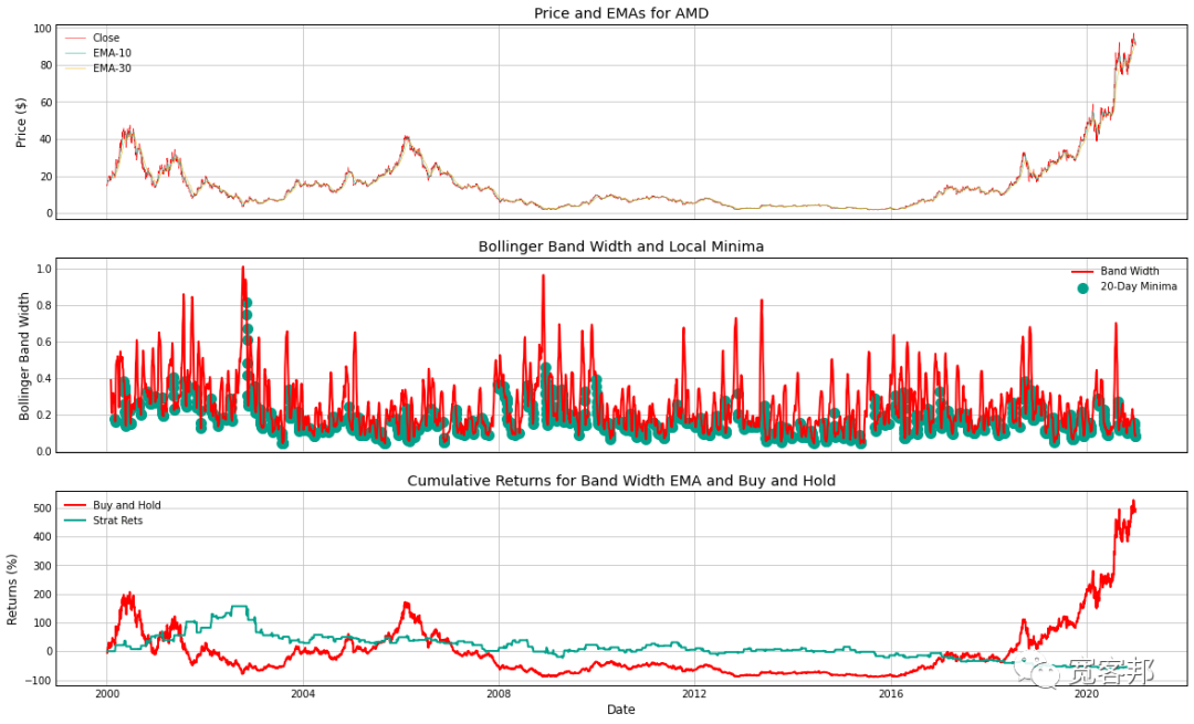
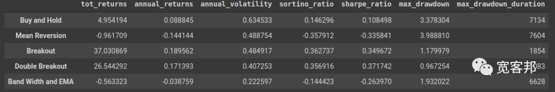
该策略在时间范围内损失了大部分启动资金,并以执行大多数其他策略而告终。我们看到的问题之一是 20 天的时间可能不够具有显著性。例如,有时带宽会上升(例如 2003、2008、2009),因此 20 天的最小值最终会升高。
例如,我们可以更新它并在进行交易之前设置一个额外的阈值,例如 20 天最小和宽度 < 0.2。我们还可以将回溯期延长至 30 天、60 天或更长时间,这将有助于我们避免在那些高波动期期间买入。当然,这一切都假设布林带在低带宽时段买入是正确的。
您可以通过多种其他方式在交易中使用布林带。您可以将其与其他指标和方法相结合,以构建比上面显示的更好策略。
扫描本文最下方二维码获取全部完整源码和Jupyter Notebook 文件打包下载。