机器学习实操(以随机森林为例)
为了展示随机森林的操作,我们用一套早期的前列腺癌和癌旁基因表达芯片数据集,包含102个样品(50个正常,52个肿瘤),2个分组和9021个变量
(基因)。(https://file.biolab.si/biolab/supp/bi-cancer/projections/info/prostata.html)
数据格式和读入数据
输入数据为标准化之后的表达矩阵,基因在行,样本在列。随机森林对数值分布没有假设。每个基因表达值用于分类时是基因内部在不同样品直接比较,只要是样品之间标准化的数据即可,其他任何线性转换如log2,scale等都没有影响 (数据在:https://gitee.com/ct5869/shengxin-baodian/tree/master/machinelearning)。
样品表达数据:
prostat.expr.txt
样品分组信息:
prostat.metadata.txt
expr_file metadata_file
# 每个基因表达值是内部比较,只要是样品之间标准化的数据即可,其它什么转换都关系不大
# 机器学习时,字符串还是默认为因子类型的好
expr_mat
# 处理异常的基因名字
rownames(expr_mat)
metadata
dim(expr_mat)

## [1] 9021  102
基因表达表示例如下:
expr_mat[1:4,1:5]

##       normal_1 normal_2 normal_3 normal_4 normal_5
## AADAC      1.3       -1       -7       -4        5
## AAK1       0.4        0       10       11        8
## AAMP      -0.4       20       -7      -14       12
## AANAT    143.3       19      397      245      328
Metadata表示例如下
head(metadata)

##           class
## normal_1 normal
## normal_2 normal
## normal_3 normal
## normal_4 normal
## normal_5 normal
## normal_6 normal

table(metadata)

## metadata
## normal  tumor
##     50     52
样品筛选和排序
对读入的表达数据进行转置。通常我们是一行一个基因,一列一个样品。在构建模型时,数据通常是反过来的,一列一个基因,一行一个样品。每一列代表一个变量
(variable),每一行代表一个案例
(case)。这样更方便提取每个变量,且易于把模型中的x,y放到一个矩阵中。
样本表和表达表中的样本顺序对齐一致也是需要确保的一个操作。
# 表达数据转置
# 习惯上我们是一行一个基因,一列一个样品
# 做机器学习时,大部分数据都是反过来的,一列一个基因,一行一个样品
# 每一列代表一个变量
expr_mat expr_mat_sampleL metadata_sampleL
common_sampleL
# 保证表达表样品与METAdata样品顺序和数目完全一致
expr_mat metadata
判断是分类还是回归
前面读数据时已经给定了参数stringsAsFactors =T,这一步可以忽略了。
# R4.0之后默认读入的不是factor,需要做一个转换
# devtools::install_github("Tong-Chen/ImageGP")
library(ImageGP)

# 此处的class根据需要修改
group = "class"

# 如果group对应的列为数字,转换为数值型 - 做回归
# 如果group对应的列为分组,转换为因子型 - 做分类
if(numCheck(metadata[[group]])){
    if (!is.numeric(metadata[[group]])) {
      metadata[[group]]     }
} else{
  metadata[[group]] }
随机森林一般分析
library(randomForest)

# 查看参数是个好习惯
# 有了前面的基础概述,再看每个参数的含义就明确了很多
# 也知道该怎么调了
# 每个人要解决的问题不同,通常不是别人用什么参数,自己就跟着用什么参数
# 尤其是到下游分析时
# ?randomForest

# 查看源码
# randomForest:::randomForest.default
加载包之后,直接分析一下,看到结果再调参。
# 设置随机数种子,具体含义见 https://mp.weixin.qq.com/s/6plxo-E8qCdlzCgN8E90zg
set.seed(304)

# 直接使用默认参数
rf
查看下初步结果,
随机森林类型判断为分类,构建了500棵树,每次决策时从随机选择的94个基因中做最优决策
(mtry),OOB估计的错误率是9.8%,挺高的。
分类效果评估矩阵Confusion matrix,显示normal组的分类错误率为0.06,tumor组的分类错误率为0.13。
rf
##
## Call:
## randomForest(x = expr_mat, y = metadata[[group]])
## Type of random forest: classification
## Number of trees: 500
## No. of variables tried at each split: 94
##
## OOB estimate of error rate: 9.8%
## Confusion matrix:
## normal tumor class.error
## normal 47 3 0.0600000
## tumor 7 45 0.1346154
随机森林标准操作流程 (适用于其他机器学习模型)
拆分训练集和测试集
library(caret)
seed set.seed(seed)
train_index train_data train_data_group
test_data test_data_group
dim(train_data)

## [1]   77 9021

dim(test_data)

## [1]   25 9021
Boruta特征选择鉴定关键分类变量
# install.packages("Boruta")
library(Boruta)
set.seed(1)

boruta        maxRuns=300)

boruta

## Boruta performed 299 iterations in 1.937513 mins.
##  46 attributes confirmed important: ADH5, AGR2, AKR1B1, ANGPT1,
## ANXA2.....ANXA2P1.....ANXA2P3 and 41 more;
##  8943 attributes confirmed unimportant: AADAC, AAK1, AAMP, AANAT, AARS
## and 8938 more;
##  32 tentative attributes left: ALDH2, ATP6V1G1, C16orf45, CDC42BPA,
## COL4A6 and 27 more;
查看下变量重要性鉴定结果(实际上面的输出中也已经有体现了),54个重要的变量,36个可能重要的变量
(tentative variable,
重要性得分与最好的影子变量得分无统计差异),6,980个不重要的变量。
table(boruta$finalDecision)

##
## Tentative Confirmed  Rejected
##        32        46      8943
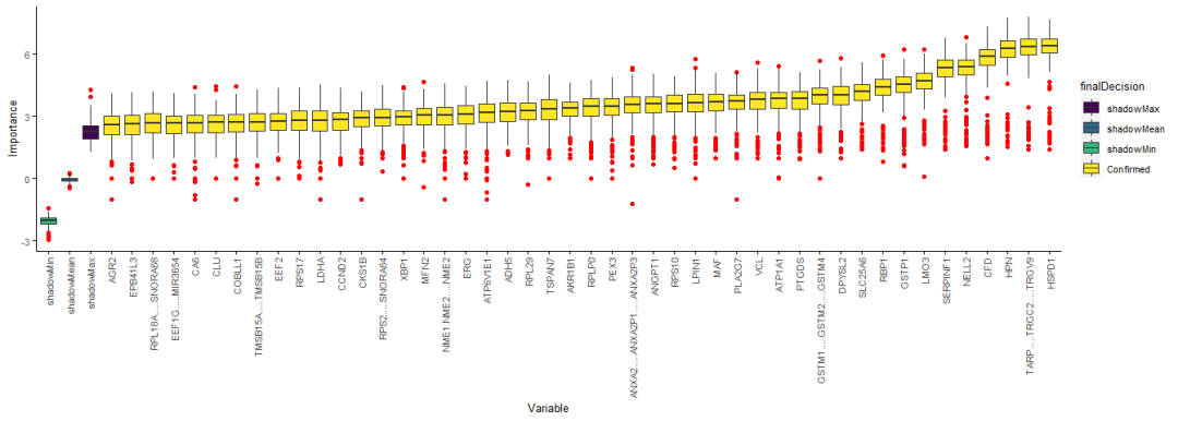
绘制鉴定出的变量的重要性。变量少了可以用默认绘图,变量多时绘制的图看不清,需要自己整理数据绘图。
定义一个函数提取每个变量对应的重要性值。
library(dplyr)
boruta.imp   imp   colnames(imp)   imp
  variableGrp                             finalDecision=x$finalDecision)

  showGrp                         finalDecision=c("shadowMax", "shadowMean", "shadowMin"))

  variableGrp
  boruta.variable.imp
  sortedVariable % group_by(Variable) %>%
    summarise(median=median(Importance)) %>% arrange(median)
  sortedVariable

  boruta.variable.imp$Variable
  invisible(boruta.variable.imp)
}

boruta.variable.imp
head(boruta.variable.imp)

##   Variable Importance finalDecision
## 1    AADAC          0      Rejected
## 2    AADAC          0      Rejected
## 3    AADAC          0      Rejected
## 4    AADAC          0      Rejected
## 5    AADAC          0      Rejected
## 6    AADAC          0      Rejected
只绘制Confirmed变量。
library(ImageGP)

sp_boxplot(boruta.variable.imp, melted=T, xvariable = "Variable", yvariable = "Importance",
           legend_variable = "finalDecision", legend_variable_order = c("shadowMax", "shadowMean", "shadowMin", "Confirmed"),
           xtics_angle = 90)
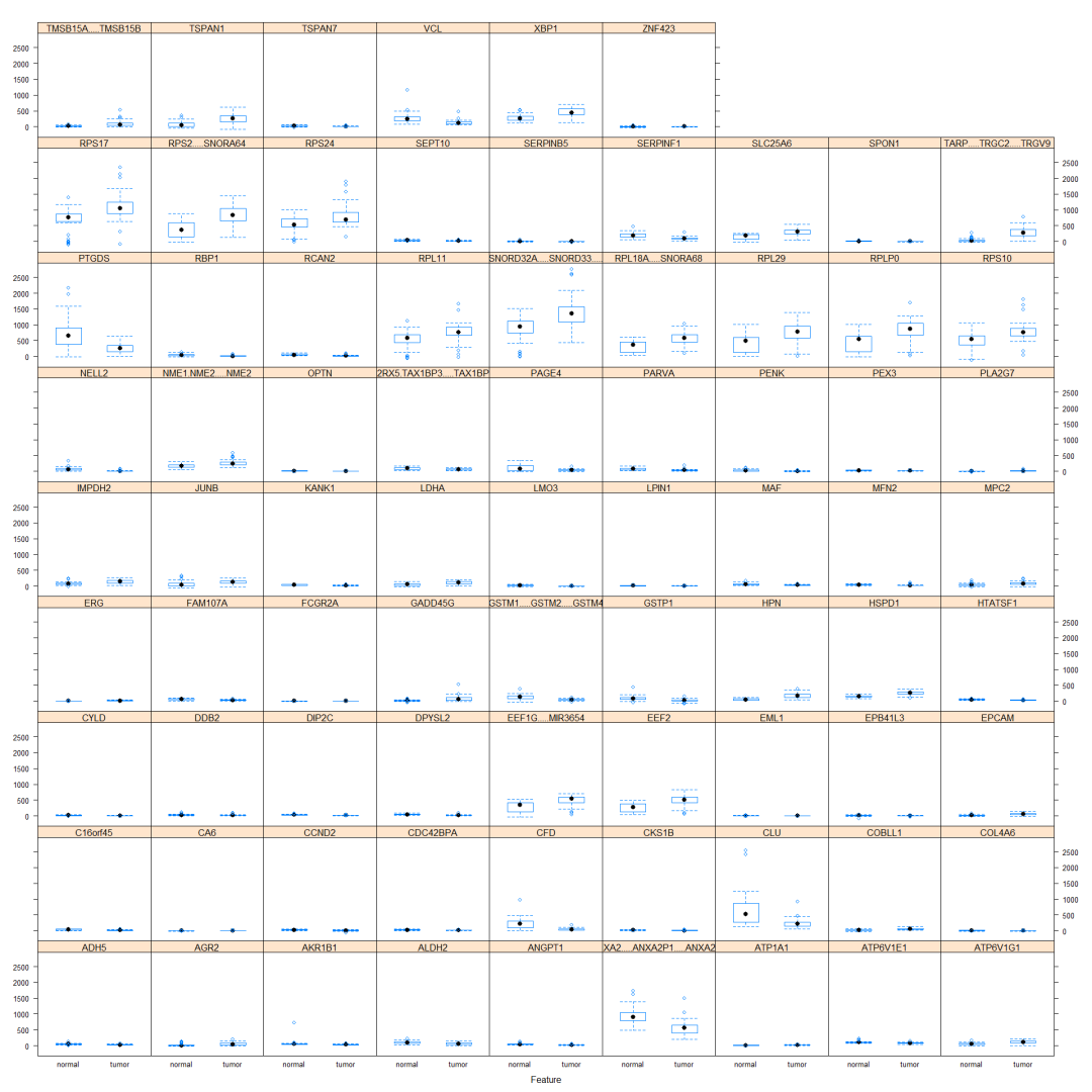
提取重要的变量和可能重要的变量
boruta.finalVarsWithTentative
看下这些变量的值的分布
caret::featurePlot(train_data[,boruta.finalVarsWithTentative$Item], train_data_group, plot="box")
交叉验证选择参数并拟合模型
定义一个函数生成一些列用来测试的mtry (一系列不大于总变量数的数值)。
generateTestVariableSet   max_power   tmp_subset   #return(tmp_subset)
  base::unique(sort(tmp_subset[tmp_subset}
# generateTestVariableSet(78)
选择关键特征变量相关的数据
# 提取训练集的特征变量子集
boruta_train_data boruta_mtry
使用 Caret 进行调参和建模
library(caret)
# Create model with default parameters
trControl
seed set.seed(seed)
# 根据经验或感觉设置一些待查询的参数和参数值
tuneGrid
borutaConfirmed_rf_default tuneGrid = tuneGrid, #
metric="Accuracy", #metric='Kappa'
trControl=trControl)
borutaConfirmed_rf_default
## Random Forest
##
## 77 samples
## 78 predictors
## 2 classes: 'normal', 'tumor'
##
## No pre-processing
## Resampling: Cross-Validated (10 fold, repeated 5 times)
## Summary of sample sizes: 71, 69, 69, 69, 69, 69, ...
## Resampling results across tuning parameters:
##
## mtry Accuracy Kappa
## 1 0.9352381 0.8708771
## 2 0.9352381 0.8708771
## 3 0.9352381 0.8708771
## 4 0.9377381 0.8758771
## 5 0.9377381 0.8758771
## 6 0.9402381 0.8808771
## 7 0.9402381 0.8808771
## 8 0.9452381 0.8908771
## 9 0.9402381 0.8808771
## 10 0.9452381 0.8908771
## 16 0.9452381 0.8908771
## 25 0.9477381 0.8958771
## 36 0.9452381 0.8908771
## 49 0.9402381 0.8808771
## 64 0.9327381 0.8658771
##
## Accuracy was used to select the optimal model using the largest value.
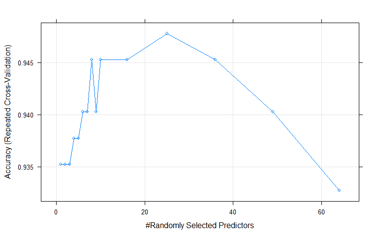
## The final value used for the model was mtry = 25.
可视化不同参数的准确性分布
plot(borutaConfirmed_rf_default)
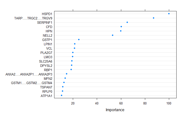
 可视化Top20重要的变量
dotPlot(varImp(borutaConfirmed_rf_default))
提取最终选择的模型,并绘制 ROC 曲线评估模型
borutaConfirmed_rf_default_finalmodel
先自评,评估模型对训练集的分类效果
采用训练数据集评估构建的模型,Accuracy=1; Kappa=1,非常完美。
模型的预测显著性P-Value [Acc > NIR] : 2.2e-16。其中NIR是No Information Rate,其计算方式为数据集中最大的类包含的数据占总数据集的比例。如某套数据中,分组A有80个样品,分组B有20个样品,我们只要猜A,正确率就会有80%,这就是NIR。如果基于这套数据构建的模型准确率也是80%,那么这个看上去准确率较高的模型也没有意义。confusionMatrix使用binom.test函数检验模型的准确性Accuracy是否显著优于NIR,若P-value<0.05,则表示模型预测准确率显著高于随便猜测。
# 获得模型结果评估矩阵(`confusion matrix`)

predictions_train confusionMatrix(predictions_train, train_data_group)

## Confusion Matrix and Statistics
##
##           Reference
## Prediction normal tumor
##     normal     38     0
##     tumor       0    39
##
##                Accuracy : 1
##                  95% CI : (0.9532, 1)
##     No Information Rate : 0.5065
##     P-Value [Acc > NIR] : < 2.2e-16
##
##                   Kappa : 1
##
##  Mcnemar's Test P-Value : NA
##
##             Sensitivity : 1.0000
##             Specificity : 1.0000
##          Pos Pred Value : 1.0000
##          Neg Pred Value : 1.0000
##              Prevalence : 0.4935
##          Detection Rate : 0.4935
##    Detection Prevalence : 0.4935
##       Balanced Accuracy : 1.0000
##
##        'Positive' Class : normal
##
盲评,评估模型应用于测试集时的效果
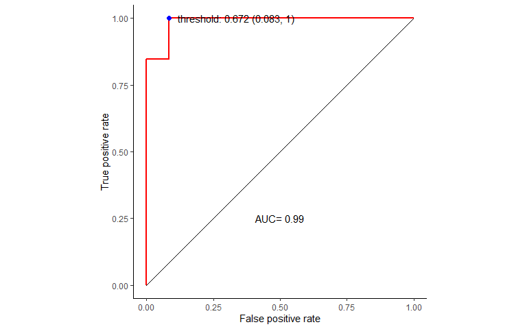
绘制ROC曲线,计算模型整体的AUC值,并选择最佳模型。
# 绘制ROC曲线

prediction_prob library(pROC)
roc_curve
roc_curve

##
## Call:
## roc.default(response = test_data_group, predictor = prediction_prob[,     1])
##
## Data: prediction_prob[, 1] in 12 controls (test_data_group normal) > 13 cases (test_data_group tumor).
## Area under the curve: 0.9872

# roc # plot(roc)
基于默认阈值的盲评
基于默认阈值绘制混淆矩阵并评估模型预测准确度显著性,结果显著P-Value [Acc > NIR]<0.05。
# 获得模型结果评估矩阵(`confusion matrix`)

predictions confusionMatrix(predictions, test_data_group)

## Confusion Matrix and Statistics
##
##           Reference
## Prediction normal tumor
##     normal     12     2
##     tumor       0    11
##
##                Accuracy : 0.92
##                  95% CI : (0.7397, 0.9902)
##     No Information Rate : 0.52
##     P-Value [Acc > NIR] : 2.222e-05
##
##                   Kappa : 0.8408
##
##  Mcnemar's Test P-Value : 0.4795
##
##             Sensitivity : 1.0000
##             Specificity : 0.8462
##          Pos Pred Value : 0.8571
##          Neg Pred Value : 1.0000
##              Prevalence : 0.4800
##          Detection Rate : 0.4800
##    Detection Prevalence : 0.5600
##       Balanced Accuracy : 0.9231
##
##        'Positive' Class : normal
##
选择模型分类最佳阈值再盲评
r是加权系数,默认是1,其计算方式为r = (1 − prevalenc**e)/(cos**t * prevalenc**e).
best.weights控制加权方式:(cost, prevalence)默认是(1,0.5),据此算出的r为1。
best_thresh                                  transpose = F, best.method = "youden"))

best_thresh$best   paste0('threshold: ', x[1], ' (', round(1-x[2],3), ", ", round(x[3],3), ")"))

best_thresh

##   threshold specificity sensitivity                        best
## 1     0.672   0.9166667           1 threshold: 0.672 (0.083, 1)
准备数据绘制ROC曲线
library(ggrepel)
ROC_data ROC_data
p   geom_step(color="red", size=1, direction = "vh") +
  geom_segment(aes(x=0, xend=1, y=0, yend=1))  + theme_classic() +
  xlab("False positive rate") +
  ylab("True positive rate") + coord_fixed(1) + xlim(0,1) + ylim(0,1) +
  annotate('text', x=0.5, y=0.25, label=paste('AUC=', round(roc_curve$auc,2))) +
  geom_point(data=best_thresh, mapping=aes(x=1-specificity, y=sensitivity), color='blue', size=2) +
  geom_text_repel(data=best_thresh, mapping=aes(x=1.05-specificity, y=sensitivity ,label=best))
p
 基于选定的最优阈值制作混淆矩阵并评估模型预测准确度显著性,结果显著
P-Value [Acc > NIR]<0.05。
predict_result
head(predict_result)

##   Predict_status Predict_class
## 1           TRUE        normal
## 2          FALSE         tumor

predictions2  best_thresh[1,1]), predict_result)

predictions2
confusionMatrix(predictions2, test_data_group)

## Confusion Matrix and Statistics
##
##           Reference
## Prediction normal tumor
##     normal     11     0
##     tumor       1    13
##
##                Accuracy : 0.96
##                  95% CI : (0.7965, 0.999)
##     No Information Rate : 0.52
##     P-Value [Acc > NIR] : 1.913e-06
##
##                   Kappa : 0.9196
##
##  Mcnemar's Test P-Value : 1
##
##             Sensitivity : 0.9167
##             Specificity : 1.0000
##          Pos Pred Value : 1.0000
##          Neg Pred Value : 0.9286
##              Prevalence : 0.4800
##          Detection Rate : 0.4400
##    Detection Prevalence : 0.4400
##       Balanced Accuracy : 0.9583
##
##        'Positive' Class : normal
##
机器学习系列教程
从随机森林开始,一步步理解决策树、随机森林、ROC/AUC、数据集、交叉验证的概念和实践。
文字能说清的用文字、图片能展示的用、描述不清的用公式、公式还不清楚的写个简单代码,一步步理清各个环节和概念。
再到成熟代码应用、模型调参、模型比较、模型评估,学习整个机器学习需要用到的知识和技能。
往期精品(点击图片直达文字对应教程)
机器学习
后台回复“生信宝典福利第一波”或点击阅读原文获取教程合集