样本分布不平衡，机器学习准确率高又有什么用？

前面无论是用全部变量还是筛选出的特征变量、无论如何十折交叉验证调参，获得的模型应用于测试集时虽然预测准确率能在90%以上，但与不基于任何信息的随机猜测相比，这个模型都是统计不显著的（这一点可能意义也不大，样本不平衡时看模型整体准确性无意义）。一个原因应该是样本不平衡导致的。DLBCL组的样品数目约为FL组的3倍。不通过建模而只是盲猜结果为DLBCL即可获得75%的正确率。而FL组的预测准确率却很低。

而通常我们关注的是占少数的样本，如是否患病，我们更希望能尽量发现可能存在的疾病，提前采取措施。

因此如何处理非平衡样品是每一个算法应用于分类问题时都需要考虑的。

不平衡样本的模型构建中的影响主要体现在2个地方：

随机采样构建决策树时会有较大概率只拿到了样品多的分类，这些树将没有能力预测样品少的分类，从而构成无意义的决策树。
在决策树的每个分子节点所做的决策会倾向于整体分类纯度，因此样品少的分类对结果的贡献和影响少。

一般处理方式有下面4种：

Class weights: 样品少的类分类错误给予更高的罚分 (impose a heavier cost when errors are made in the minority class)
Down-sampling: 从样品多的类随机移除样品
Up-sampling: 在样品少的类随机复制样品 (randomly replicate instances in the minority class)
Synthetic minority sampling technique (SMOTE): 通过插值在样品少的类中合成填充样本

这些权重加权或采样技术对阈值依赖的评估指标如准确性等影响较大，它们相当于把决策阈值推向了ROC曲线中的”最优位置” (这在Boruta特征变量筛选部分有讲)。但这些权重加权或采样技术对ROC曲线通常影响不会太大。

基于模拟数据的样本不平衡处理

这里先通过一套模拟数据熟悉下处理流程，再应用于真实数据。采用caret包的twoClassSim函数生成包含20个有意义变量和10个噪音变量的数据集。该数据集包含5000个观察样品，分为两组，多数组和少数组的样品数目比例为50:1 (通过intercept参数控制)。

library(dplyr) # for data manipulation
library(caret) # for model-building
# install.packages("xts")
# install.packages("quantmod")
# wget https://cran.r-project.org/src/contrib/Archive/DMwR/DMwR_0.4.1.tar.gz
# R CMD INSTALL DMwR_0.4.1.tar.gz
library(DMwR) # for smote implementation 
# 或使用smotefamily代替
# library(smotefamily) # for smote implementation
library(purrr) # for functional programming (map)
library(pROC) # for AUC calculations

set.seed(2969)

imbal_train                            intercept = -25,
                           linearVars = 20,
                           noiseVars = 10)

imbal_train$Class = ifelse(imbal_train$Class == "Class1", "Normal", "Disease")
imbal_train$Class 
imbal_test                             intercept = -25,
                           linearVars = 20,
                           noiseVars = 10)
imbal_test$Class = ifelse(imbal_test$Class == "Class1", "Normal", "Disease")
imbal_test$Class 
prop.table(table(imbal_train$Class))

prop.table(table(imbal_test$Class))

样品构成

Disease  Normal 
 0.0204  0.9796 

Disease  Normal 
 0.0252  0.9748

构建原始GBM模型

这里应用另外一种集成学习算法 (GBM, Gradient Boosting Machine)进行模型构建。GBM也是效果很好的集成学习算法，可以处理变量的互作和非线性关系。机器学习中常用的GBDT、XGBoost和LightGBM算法（或工具）都是基于梯度提升机（GBM）的算法思想。

先构建一个原始模型，重复5次10-折交叉验证寻找最优的模型超参数，采用AUC作为评估标准。这些概念如果不熟悉翻一下往期推文。

# Set up control function for training
ctrl                      number = 10,
                     repeats = 5,
                     summaryFunction = twoClassSummary,
                     classProbs = TRUE)

# Build a standard classifier using a gradient boosted machine

set.seed(5627)
orig_fit                   data = imbal_train,
                  method = "gbm",
                  verbose = FALSE,
                  metric = "ROC",
                  trControl = ctrl)

# Build custom AUC function to extract AUC
# from the caret model object

test_roc   roc(data$Class,
      predict(model, data, type = "prob")[, "Disease"])

}

orig_fit %>%
  test_roc(data = imbal_test) %>%
  auc()

AUC值为0.95，还是很不错的。

Setting levels: control = Disease, case = Normal
Setting direction: controls > cases
Area under the curve: 0.9538

从confusion matrix (预测结果采用默认阈值)来看，Disease的分类效果一般，准确率（敏感性）只有30.6%。不管是Normal还是Disease都倾向于预测为Normal,特异性低，这是因为样品不平衡导致的。而我们通常更希望尽早发现疾病的存在。

predictions_train confusionMatrix(predictions_train, imbal_test$Class)

Confusion Matrix and Statistics

          Reference
Prediction Disease Normal
   Disease      38     17
   Normal       88   4857

               Accuracy : 0.979           
                 95% CI : (0.9746, 0.9828)
    No Information Rate : 0.9748          
    P-Value [Acc > NIR] : 0.02954         

                  Kappa : 0.4109          




    
 Mcnemar's Test P-Value : 8.415e-12       

            Sensitivity : 0.3016          
            Specificity : 0.9965          
         Pos Pred Value : 0.6909          
         Neg Pred Value : 0.9822          
             Prevalence : 0.0252          
         Detection Rate : 0.0076          
   Detection Prevalence : 0.0110          
      Balanced Accuracy : 0.6490          

       'Positive' Class : Disease

采用权重分配或抽样方式处理样品不平衡问题

这里应用的GBM模型自身有一个参数weights可以用于设置样品的权重；caret在trainControl函数中提供了sampling参数可以进行up-sample和down-sample，或其它任何算法的采样方式(这里用的是smotefamily::SMOTE函数进行采样)。

# Create model weights (they sum to one)
# 给每一个观察一个权重
class1_weight = (1/table(imbal_train$Class)[['Normal']]) * 0.5
class2_weight = (1/table(imbal_train$Class)[["Disease"]]) * 0.5
model_weights                         class1_weight, class2_weight)

# Use the same seed to ensure same cross-validation splits
ctrl$seeds 
# Build weighted model

weighted_fit                       data = imbal_train,
                      method = "gbm",
                      verbose = FALSE,
                      weights = model_weights,
                      metric = "ROC",
                      trControl = ctrl)

# Build down-sampled model

ctrl$sampling 
down_fit                   data = imbal_train,
                  method = "gbm",
                  verbose = FALSE,
                  metric = "ROC",
                  trControl = ctrl)

# Build up-sampled model

ctrl$sampling 
up_fit                 data = imbal_train,
                method = "gbm",
                verbose = FALSE,
                metric = "ROC",
                trControl = ctrl)

# Build smote model
ctrl$sampling 
smote_fit                    data = imbal_train,
                   method = "gbm",
                   verbose = FALSE,
                   metric = "ROC",
                   trControl = ctrl)

计算下每个模型的AUC值

# Examine results for test set

model_list                    weighted = weighted_fit,
                   down = down_fit,
                   up = up_fit,
                   SMOTE = smote_fit)

model_list_roc %
  map(test_roc, data = imbal_test)

model_list_roc %>%
  map(auc)

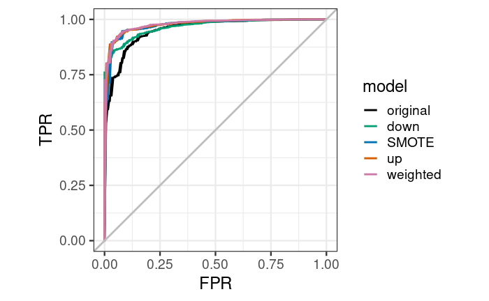
样品加权模型获得的AUC值最高，其次是up-sample, SMOTE, down-sample，结果都比original有提高。

Setting levels: control = Disease, case = Normal
Setting direction: controls > cases
Setting levels: control = Disease, case = Normal
Setting direction: controls > cases
Setting levels: control = Disease, case = Normal
Setting direction: controls > cases
Setting levels: control = Disease, case = Normal
Setting direction: controls > cases
Setting levels: control = Disease, case = Normal
Setting direction: controls > cases
$original
Area under the curve: 0.9538

$weighted
Area under the curve: 0.9793

$down
Area under the curve: 0.9667

$up
Area under the curve: 0.9778

$SMOTE
Area under the curve: 0.9744

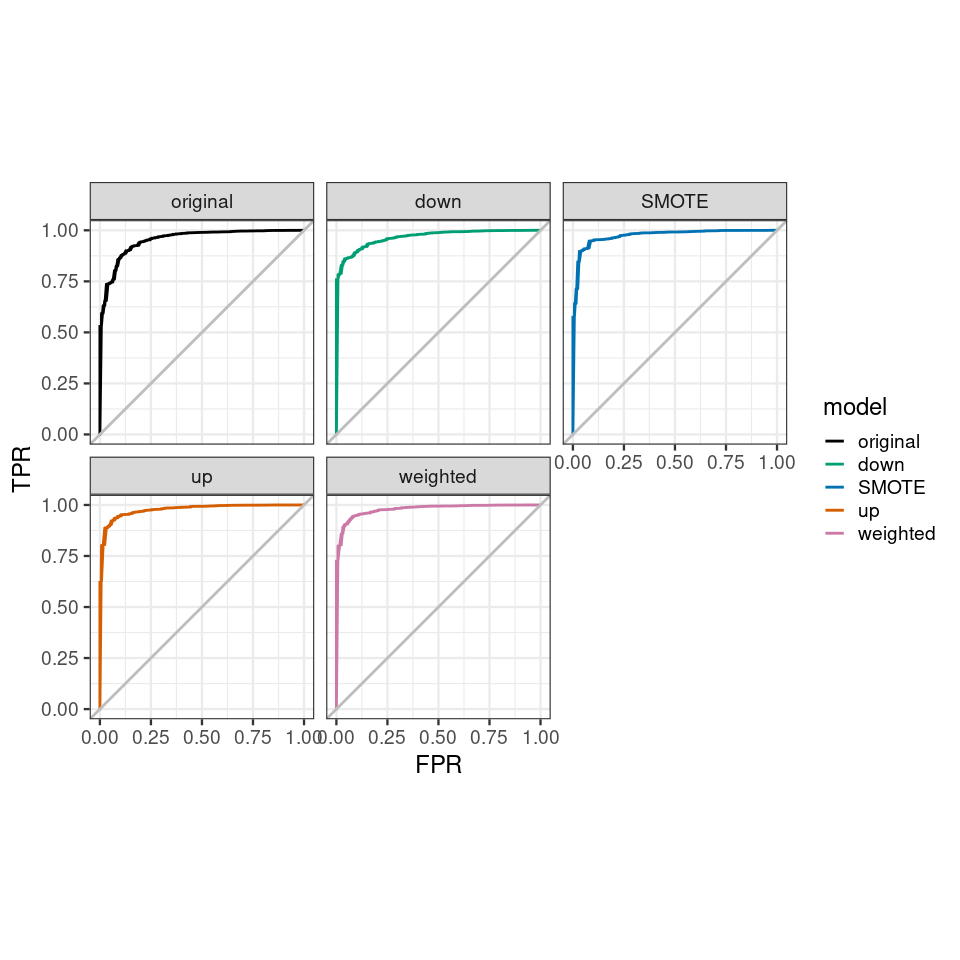
绘制下ROC曲线，查看下模型的具体效果展示。样品加权的模型优于其它所有模型，原始模型在假阳性率0-25%时效果差于其它模型。好的模型是在较低假阳性率时具有较高的真阳性率。

results_list_roc num_mod 
for(the_roc in model_list_roc){

  results_list_roc[[num_mod]]     data_frame(TPR = the_roc$sensitivities,
               FPR = 1 - the_roc$specificities,
               model = names(model_list)[num_mod])

  num_mod 
}

results_df_roc 
results_df_roc$model                                levels=c("original", "down","SMOTE","up","weighted"))

# Plot ROC curve for all 5 models

custom_col 
ggplot(aes(x = FPR,  y = TPR, group = model), data = results_df_roc) +
  geom_line(aes(color = model), size = 1) +
  scale_color_manual(values = custom_col) +
  geom_abline(intercept = 0, slope = 1, color = "gray", size = 1) +
  theme_bw(base_size = 18) + coord_fixed(1)

ggplot(aes(x = FPR,  y = TPR, group = model), data = results_df_roc) +
  geom_line(aes(color = model), size = 1) +
  facet_wrap(vars(model)) +
  scale_color_manual(values = custom_col) +
  geom_abline(intercept = 0, slope = 1, color = "gray", size = 1) +
  theme_bw(base_size = 18) + coord_fixed(1)

加权后的模型，总预测准确率降低了一点，但Disease的预测准确性升高了2.47倍，70.63%。

predictions_train confusionMatrix(predictions_train, imbal_test$Class)

结果如下




    
Confusion Matrix and Statistics

          Reference
Prediction Disease Normal
   Disease      89     83
   Normal       37   4791

               Accuracy : 0.976           
                 95% CI : (0.9714, 0.9801)
    No Information Rate : 0.9748          
    P-Value [Acc > NIR] : 0.3137          

                  Kappa : 0.5853          

 Mcnemar's Test P-Value : 3.992e-05       

            Sensitivity : 0.7063          
            Specificity : 0.9830          
         Pos Pred Value : 0.5174          
         Neg Pred Value : 0.9923          
             Prevalence : 0.0252          
         Detection Rate : 0.0178          
   Detection Prevalence : 0.0344          
      Balanced Accuracy : 0.8447          

       'Positive' Class : Disease