“ 快速高效学会python的终极奥义：过、抄、仿、改、调、看、练、创、悟”

正文开始前，首先声明下，我也是半路出家非科班出身，所以可能代码的规范

上一课我们大概学习了python的基本代码，最后一个部分，我们提到python相比于其他的编程语言，最实用也是最有魅力的地方就在于你可以找到各种各样的包包，他们几乎可以满足你所有的需求，非常适合不喜欢自己造轮子，喜欢抄代码的人比如我，如果你有一些定制化的需求，代码也都是开源的，可以自己扒拉下来再手动做一些修改，大大节约了工作量。

—

开始之前你需要了解的

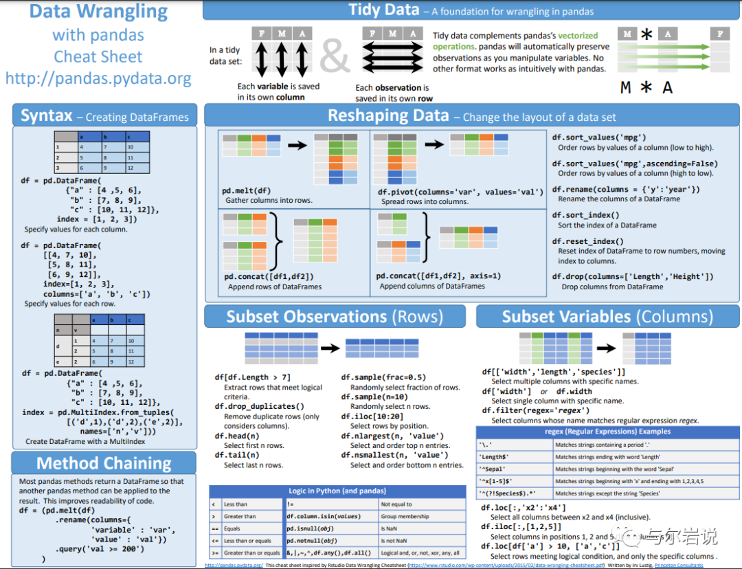
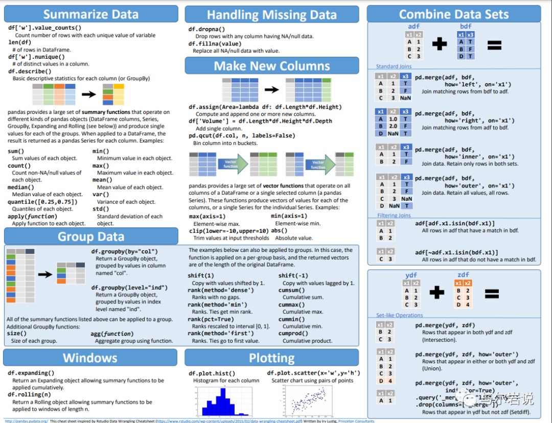
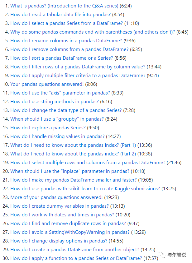
今天主要介绍的就是做数据分析必不可少的一个包包，pandas，这里给大家吐血安利youtube上的一系列视频，是我自己觉得在市面上翻出来最实用的一套课，每个短片都控制在10分钟之内，想要真正学好的可以大致看一看，如果想偷懒，可以直接看我的精华提炼版本，然后代码也不用都记住，只要用的时候翻到我的帖子，然后全文搜索下，再ctrl C大法好粘贴过去，我把视频里面提到的方法全都汇总在下面了，方便大家copy~~~

微信没办法粘贴外链过来，就直接手动贴一个，其他都在这个目录底下~

https://www.youtube.com/watch?v=yzIMircGU5I&list=PL5-da3qGB5ICCsgW1MxlZ0Hq8LL5U3u9y&index=2

https://pandas.pydata.org/docs/user_guide/index.html#user-guide

跟上节课一样，我还是习惯先肢解下课程内容，其实pandas你就想成学excel就好，excel的基本操作有什么，pandas就基本有什么，那excel的功能大致上有：数据转换（导入各种文件类型，生成各种文件类型）、表格建立和编辑（包括绝对位置和相对位置的取数、增删行、列，两个表格横着竖着拼接等等）、数据分析和处理（包括数据透视表、各种函数、画各种图表），pandas的功能也基本就是这些，有更细致的需求，直接百度或者在我的文章里关键词检索，然后copy代码就可以，基本的操作只需要掌握这些。照例有需要的朋友可以转发+后台留言，我给大家发课后的代码，可以自己再练习~~

—

基本内容学习

第一步永远是导入包包




    
from pandas import Series, DataFrame
import pandas as pd

参考：
https://amaozhao.gitbooks.io/pandas-notebook/content/
https://github.com/justmarkham/pandas-videos/blob/master/pandas.ipynb

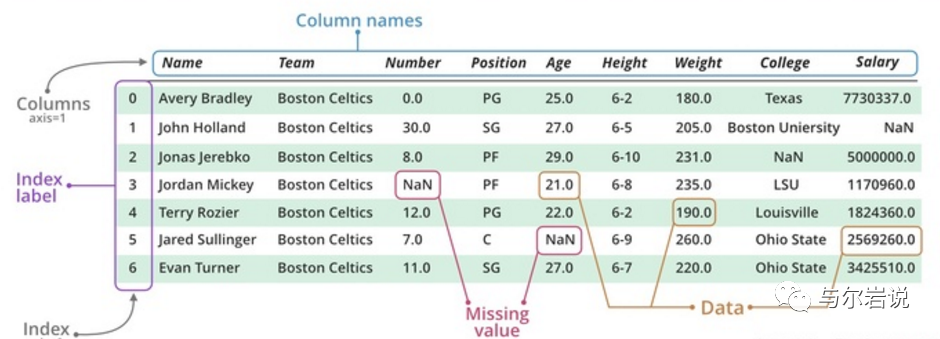
pandas的数据类型

有两类，一种是dataframe一种是series，其中dataframe是多行多列，而series是单列多行，其都有行和列组成。

创建series和dataframe

1.创建series

通过列表创建

obj = Series([4, 7, -5, 3]) 
obj2 = Series([4, 7, -5, 3], index=['d','b','a','c']) #指定索引

通过字典创建

sdata = {'Ohio':35000, 'Texas':7100, 'Oregon':1600,'Utah':500}
obj3 = Series(sdata)

通过字典加索引

states = ['California', 'Ohio', 'Oregon', 'Texas']
obj4 = Series(sdata, index=states)

2.创建dataframe

词典生成

data = {'state':['Ohio', 'Ohio', 'Ohio', 'Nevada','Nevada'],
        'year':[2000, 2001, 2002, 2011, 2002],
        'pop':[1.5, 1.7, 3.6, 2.4, 2.9]}
frame = DataFrame(data)
frame2 = DataFrame(data, columns=['year', 'state', 'pop']) #指定列
frame3 = DataFrame(data, columns=['year', 'state', 'pop']，
         index=['one', 'two', 'three', 'four', 'five']) #指定列和索引

列表生成（常用）

errors = [('c',1,'right'), ('b', 2,'wrong')]
df = pd.DataFrame(errors，columns=['name', 'count', 'result'])

嵌套词典

pop = {'Nevada':{2001:2.4, 2002:2.9},
       'Ohio':{2000:1.5, 2001:1.7, 2002


    
:3.6}}
frame4 = DataFrame(pop)
Out[138]:
      Nevada  Ohio
2000     NaN   1.5
2001     2.4   1.7
2002     2.9   3.6

series组合

In [4]: a = pd.Series([1,2,3]) 
In [5]: b = pd.Series([2,3,4])
In [6]: c = pd.DataFrame([a,b]) 
In [7]: c
Out[7]:
   0  1  2
0  1  2  3
1  2  3  4
#或者也可以按照列来生成dataframe
c = pd.DataFrame({'a':a,'b':b})

读取数据

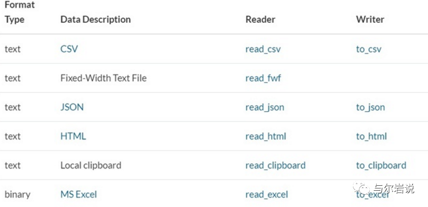
pandas可以读取多种数据类型，包括但是不限于csv、txt、xlsx、json、html、sql等等，只有你想不到没有他不能读，一般读取通过read_xxx输出通过to_xxx

索引和选取

对于一组数据：

data = DataFrame(np.arange(16).reshape((4,4)),index=['Ohio', 'Colorado','Utah','New York'],columns=['one','two','three','four'])
>>> data
          one  two  three  four
Ohio        0    1      2     3
Colorado    4    5      6     7
Utah        8    9     10    11
New York   12   13     14    15

几种索引方式

事实上有很多种索引方式，ix是较老的方式

data['two']
data.ix['Ohio']
data.ix['Ohio', ['two','three']]

较新的是loc与iloc
loc用于索引中有文字的，iloc仅仅用于索引为数字的
然后比较坑的是经常是索引不成功，
对于列来说：这时候要检查下这个名字对不对？可以用
data.columns=[]来强行规定名字然后再索引
对于行来说：可以强行reset_index或者set_index为新的一组值，基本可以避免大坑

按照索引来遍历

按照行来进行，这个操作其实很低效率

lbsdata=pd.read_csv('testlocation.csv',sep='\t')
lbstagRow = pd.DataFrame()
lbstag = pd.DataFrame()
for


    
 index, row in lbsdata.iterrows():
    lbstagRow['recommend'] = [jsonToSp['formatted_address']]
    lbstagRow['city'] = [jsonToSparse['addressComponent']]
    lbstag = lbstag.append(lbstagRow,ignore_index=True)

也可以：

for ix, row in df.iterrows():
for ix, col in df.iteritems():
for i in range(0,len(df)):

排序

按列排序

In[73]: obj = Series(range(4), index=['d','a','b','c'])
In[74]: obj.sort_index()  
Out[74]: 
a    1
b    2
c    3
d    0
dtype: int64
In[78]: frame = DataFrame(np.arange(8).reshape((2,4)),index=['three', 'one'],columns=['d','a','b','c'])
In[79]: frame
Out[79]: 
       d  a  b  c
three  0  1  2  3
one    4  5  6  7
In[86]: frame.sort_index()
Out[86]: 
       d  a  b  c
one    4  5  6  7
three  0  1  2  3
In[87]: frame.sort()
Out[87]: 
       d  a  b  c
one    4  5  6  7
three  0  1  2  3

按行排序

In[89]: frame.sort_index(axis=1, ascending=False)
Out[89]: 
       d  c  b  a
three  0  3  2  1
one    4  7  6  5

按值排序

frame.sort_values('a')

删除

删除指定轴上的项

即删除 Series 的元素或 DataFrame 的某一行（列）的意思，通过对象的 .drop(labels, axis=0) 方法：

In[11]: ser = Series([4.5,7.2,-5.3,3.6], index=['d','b','a','c'])
In[13]: ser.drop('c')
Out[13]: 
d    4.5
b    7.2
a   -5.3
dtype: float64

删除行和列

In[17]: df = DataFrame(np.arange(9).reshape(3,3), index=['a','c','d'], columns=['oh','te','ca'])
In[18]: df
Out[18]: 
   oh  te  ca
a   0   1   2
c   3   4   5
d   6   7   8
In[19]: df.drop('a')
Out[19]: 
   oh  te  ca
c   3   4   5
d   6   7   8
In[20]: df.drop(['oh','te'],axis=1)
Out[20]: 
   ca
a   2
c   5
d   8

删除点

df_train.sort_values(by = 'GrLivArea',ascending = False)[:2]
df_train = df_train.drop(df_train[df_train['Id'] == 1299].index)
df_train = df_train.drop(df_train[df_train['Id'] == 524].index)

DataFrame连接

算术运算

In[5]: df1 = DataFrame(np.arange(12.).reshape((3,4)),columns=list('abcd'))
In[6]: df2 = DataFrame(np.arange(20.).reshape((4,5)),columns=list('abcde'))
In[9]: df1+df2
Out[9]: 
    a   b   c   d   e
0   0   2   4   6 NaN
1   9  11  13  15 NaN
2  18  20  22  24 NaN
3 NaN NaN NaN NaN NaN
# 传入填充值
In[11]: df1.add(df2, fill_value=0)
Out[11]: 
    a   b   c   d   e
0   0   2   4   6   4
1   9  11  13  15   9
2  18  20  22  24  14
3  15  16  17  18  19

merge

pandas.merge可根据一个或多个键将不同DataFrame中的行连接起来。

默认情况下，merge做的是“inner”连接，结果中的键是交集，其它方式还有“left”，“right”，“outer”。“outer”外连接求取的是键的并集，组合了左连接和右连接。

In[14]: df1 = DataFrame({'key':['b','b','a','c','a','a','b'],'data1':range(7)})
In[15]: df2 = DataFrame({'key':['a','b','d'],'data2':range(3)})
In[18]: pd.merge(df1, df2)  #或显式: pd.merge(df1, df2, on='key')
Out[18]: 
   data1 key  data2
0      0   b      1
1      1   b      1
2      6   b      1
3      2   a      0
4      4   a      0
5      5   a      0

concat

这种数据合并运算被称为连接（concatenation）、绑定（binding）或堆叠（stacking）。默认情况下，concat是在axis=0（行）上工作的，最终产生一个新的Series。如果传入axis=1（列），则变成一个DataFrame。

pd.concat([s1,s2,s3], axis=1)
dfs = []
for classify in classify_finance + classify_other:
    sql = "select classify, tags from {} where classify='{}' length(tags)>0 limit 1000".format(mysql_table_sina_news_all, classify)
    df = pd.read_sql(sql,engine)
    dfs.append(df)
df_all = pd.concat(dfs, ignore_index=True)

数据转换

数据过滤、清理以及其他的转换工作。

移除重复数据（去重）

duplicated()
DataFrame的duplicated方法返回一个布尔型Series，表示各行是否是重复行

df = DataFrame({'k1':['one']*3 + ['two']*4, 'k2':[1,1,2,3,3,4,4]})
df.duplicated()
df.drop_duplicates()

利用函数或映射进行数据转换

对于数据:

df = DataFrame({'food':['bacon','pulled pork','bacon','Pastraml','corned beef', 'Bacon', 'pastraml','honey ham','nova lox'],'ounces':[4,3,12,6,7.5,8,3,5,6]})

增加一列表示该肉类食物来源的动物类型，先编写一个肉类到动物的映射：

meat_to_animal = {'bacon':'pig',
    'pulled pork':'pig',
    'pastraml':'cow',
    'corned beef':'cow',
    'honey ham':'pig',
    'nova lox':'salmon'}

map

Series的map方法可以接受一个函数或含有映射关系的字典型对象。

df['animal'] = df['food'].map(str.lower).map(meat_to_animal)
df['food'].map(lambda x : meat_to_animal[x.lower()])
Out[22]: 
0       pig
1       pig
2       pig
3       cow
4       cow
5       pig
6       cow
7       pig
8    salmon

apply 和 applymap

对于DataFrame：

In[21]: df = DataFrame(np.random.randn(4,3), columns=list('bde'),index=['Utah','Ohio','Texas','Oregon'])
In[22]: df
Out[22]: 
               b         d         e
Utah    1.654850  0.594738 -1.969539
Ohio    2.178748  1.127218  0.451690
Texas   1.209098 -0.604432 -1.178433
Oregon  0.286382


    
  0.042102 -0.345722

apply将函数应用到由各列或行所形成的一维数组上。

作用到列：

In[24]: f = lambda x : x.max() - x.min()
In[25]: df.apply(f)
Out[25]: 
b    1.892366
d    1.731650
e    2.421229
dtype: float64

作用到行

In[26]: df.apply(f, axis=1)
Out[26]: 
Utah      3.624390
Ohio      1.727058
Texas     2.387531
Oregon    0.632104
dtype: float64

作用到每个元素

In[70]: frame = DataFrame(np.random.randn(4,3), columns=list('bde'),index=['Utah','Ohio','Texas','Oregon'])
In[72]: frame.applymap(lambda x : '%.2f' % x)
Out[72]: 
            b      d      e
Utah     1.19   1.56  -1.13
Ohio     0.10  -1.03  -0.04
Texas   -0.22   0.77  -0.73
Oregon   0.22  -2.06  -1.25

numpy的ufuncs
Numpy的ufuncs（元素级数组方法）也可用于操作pandas对象。
取绝对值操作np.abs(),np.max(),np.min()

替换值

In[23]: se = Series([1, -999, 2, -999, -1000, 3])
In[24]: se.replace(-999, np.nan)
Out[24]: 
0       1
1     NaN
2       2
3     NaN
4   -1000
5       3
dtype: float64
In[25]: se.replace([-999, -1000], np.nan)
Out[25]: 
0     1
1   NaN
2     2
3   NaN
4   NaN
5     3
dtype: float64
In[26]: se.replace([-999, -1000], [np.nan, 0])
Out[26]: 
0     1
1   NaN
2     2
3   NaN
4     0
5     3
dtype: float64
# 字典
In[27]: se.replace({-999:np.nan, -1000:0})



    
Out[27]: 
0     1
1   NaN
2     2
3   NaN
4     0
5     3
dtype: float64

df.rename(index=str.title, columns=str.upper)
df.rename(index={'OHIO':'INDIANA'}, columns={'three':'peekaboo'})

离散化和面元划分

pd.cut

为了便于分析，连续数据常常离散化或拆分为“面元”（bin）。比如：

ages = [20, 22,25,27,21,23,37,31,61,45,41,32]

需要将其划分为“18到25”, “26到35”，“36到60”以及“60以上”几个面元。要实现该功能，需要使用pandas的cut函数。

bins = [18, 25, 35, 60, 100]
cats = pd.cut(ages, bins)
Out[39]: 
[(18, 25], (18, 25], (18, 25], (25, 35], (18, 25], ..., (25, 35], (60, 100], (35, 60], (35, 60], (25, 35]]
Length: 12
Categories (4, object): [(18, 25] < (25, 35] < (35, 60] < (60, 100]]

可以通过right=False指定哪端是开区间或闭区间。也可以指定面元的名称：

cats = pd.cut(ages, bins, right=False)
group_name = ['Youth', 'YoungAdult', 'MiddleAged', 'Senior']
cats = pd.cut(ages, bins, labels=group_name)
pd.value_counts(cats)
Out[46]: 
Youth         5
MiddleAged    3
YoungAdult    3
Senior        1
dtype: int64

pd.qcut

qcut是一个非常类似cut的函数，它可以根据样本分位数对数据进行面元划分，根据数据的分布情况，cut可能无法使各个面元中含有相同数量的数据点，而qcut由于使用的是样本分位数，可以得到大小基本相等的面元。

In[48]: data = np.random.randn(1000)
In[49]: cats = pd.qcut(data, 4)
In[50]: cats
Out[50]: 
[(0.577, 3.564], (-0.729, -0.0341], (-0.729, -0.0341], (0.577, 3.564], (0.577, 3.564], ..., [-3.0316, -0.729], [-3.0316, -0.729], (-0.0341, 0.577], [-3.0316, -0.729], (-0.0341, 0.577]]
Length: 1000
Categories (4, object): [[-3.0316, -0.729] < (-0.729, -0.0341] < (-0.0341, 0.577] < (0.577, 3.564]]
In[51]: pd.value_counts(cats)
Out[51]: 
(0.577, 3.564]       250
(-0.0341, 0.577]     250
(-0.729, -0.0341]    250
[-3.0316, -0.729]    250
dtype: int64

检测和过滤异常值

可以先describe然后在找出超过某一个阈值的

data[(np.abs(data)>3).any(1)]
data[np.abs(data)>3] = np.sign(data)*3
In[63]: data.describe()
Out[63]: 
                 0            1            2            3
count  1000.000000  1000.000000  1000.000000  1000.000000
mean     -0.067623     0.068473     0.025153    -0.002081
std       0.995485     0.990253     1.003977     0.989736
min      -3.000000    -3.000000    -3.000000    -3.000000
25%      -0.774890    -0.591841    -0.641675    -0.644144
50%      -0.116401     0.101143     0.002073    -0.013611



    
75%       0.616366     0.780282     0.680391     0.654328
max       3.000000     2.653656     3.000000     3.000000

单因素分析

这里的关键在于如何建立阈值，定义一个观察值为异常值。我们对数据进行正态化，意味着把数据值转换成均值为0，方差为1的数据。

saleprice_scaled= StandardScaler().fit_transform(df_train['SalePrice'][:,np.newaxis]);
low_range = saleprice_scaled[saleprice_scaled[:,0].argsort()][:10]
high_range= saleprice_scaled[saleprice_scaled[:,0].argsort()][-10:]
print('outer range (low) of the distribution:')
print(low_range)
print('\nouter range (high) of thedistribution:')
print(high_range)

进行正态化后，可以看出：

低范围的值都比较相似并且在0附近分布。
高范围的值离0很远，并且七点几的值远在正常范围之外。

双变量分析

'GrLivArea'和'SalePrice'双变量分析

var = 'GrLivArea'
data = pd.concat([df_train['SalePrice'], df_train[var]], axis=1)
data.plot.scatter(x=var, y='SalePrice', ylim=(0,800000));

正态性：

应主要关注以下两点：
直方图 - 峰度和偏度。
正态概率图 - 数据分布应紧密跟随代表正态分布的对角线。

‘SalePrice’

绘制直方图和正态概率图：

sns.distplot(df_train['SalePrice'], fit=norm);
fig = plt.figure()
res = stats.probplot(df_train['SalePrice'], plot=plt)

可以看出，房价分布不是正态的，显示了峰值，正偏度，但是并不跟随对角线。
可以用对数变换来解决这个问题

进行对数变换：

df_train['SalePrice']= np.log(df_train['SalePrice'])

绘制变换后的直方图和正态概率图：

sns.distplot(df_train['SalePrice'], fit=norm);
fig = plt.figure()
res = stats.probplot(df_train['SalePrice'], plot=plt)

同方差性：

最好的测量两个变量的同方差性的方法就是图像。

'SalePrice' 和 'GrLivArea'同方差性

绘制散点图：
plt.scatter(df_train['GrLivArea'],df_train['SalePrice']);

虚拟变量

将类别变量转换为虚拟变量：
df_train = pd.get_dummies(df_train)

def factor(series):
    levels = list(set(series))
    design_matrix = np.zeros((len(series), len(levels)))
    for row_index, elem in enumerate(series):
        design_matrix[row_index, levels.index(elem)] = 1
    name = series.name or ""
    columns = map(lambda level: "%s[%s]" % (name, level), levels)
    df = pd.DataFrame(design_matrix, index=series.index,
                      columns=columns)
    return df

在处理类别变量的时候可以：

data.apply(lambda x: sum(x.isnull()))
var = ['Gender','Salary_Account','Mobile_Verified','Var1','Filled_Form','Device_Type','Var2','Source']
for v in var:
    print '\nFrequency count for variable %s'%v
    print data[v].value_counts()
print len(data['City'].unique())
#drop city because too many unique
data.drop('City',axis=1,inplace=True)

更加简单的方法是：

from sklearn.preprocessing import LabelEncoder
le = LabelEncoder()
var_to_encode = ['Device_Type','Filled_Form','Gender','Var1','Var2','Mobile_Verified','Source']
for col in var_to_encode:
    data[col] = le.fit_transform(data[col])
data = pd.get_dummies(data, columns=var_to_encode)
data.columns

处理时间变量

data['Age'] = data['DOB'].apply(lambda x: 115 - int(x[-2:]))
data['Age'].head()

df_train.onlineDate=pd.to_datetime(df_train.onlineDate)
df_train['age']=(datetime.date.today()-df_train.onlineDate).dt.days

词向量化

# import and init CountVectorizer
from sklearn.feature_extraction.text import CountVectorizer

vectorizer = CountVectorizer()
vectorizer # default parameters

CountVectorizer(analyzer='word', binary=False, decode_error='strict',
        dtype='numpy.int64'>, encoding='utf-8', input='content',
        lowercase=True, max_df=1.0, max_features=None, min_df=1,
        ngram_range=(1, 1), preprocessor=None, stop_words=None,
        strip_accents=None, token_pattern='(?u)\\b\\w\\w+\\b',
        tokenizer=None, vocabulary=None)
# transform text into document-term matrix

X = vectorizer.fit_transform(reviews)
print(type(X)) # X is a sparse matrix
print(X)

处理百分号

p_float = df['p_str'].str.strip("%").astype(float)/100;
p_float_2 = p_float.round(decimals=2)

p_str_2 = p_float.apply(lambda x: format(x, '.2%'));

特征离散化

s_amount_C = df_lc_C['借款金额']
q = [0.05, 0.2, 0.5, 0.8, 0.95]
bins = s_amount_C.quantile(q)
s_fea_dct_amount_C = pd.cut(s_amount_C, add_ends_to_bins(bins.values))
dict_s_fea_dct['amount'] = s_fea_dct_amount_C

s_term_C = df_lc_C['借款期限']
q = [0.05, 0.2, 0.5, 0.8, 0.95]
bins = s_term_C.quantile(q)
sns.countplot(s_term_C);

看有多少个类别




    
def add_ends_to_bins(bins):
    return np.append(np.insert(bins, 0, -np.inf), np.inf)
    
df_lc_C.groupby(s_type_C).size()
for col in category:
print(df_train2[str(col)].value_counts(dropna=False))
sns.countplot(s_is_first_C);

处理不同类别变量

DataFrame.convert_objects(convert_dates=True, convert_numeric=False, convert_timedeltas=True, copy=True)
这个命令非常好用！

使效率倍增的Pandas使用技巧

本文取自Analytics Vidhya的一个帖子12 Useful Pandas Techniques in Python for Data Manipulation，浏览原帖可直接点击链接，中文版可参见Datartisan的用 Python 做数据处理必看：12 个使效率倍增的 Pandas 技巧。这里主要对帖子内容进行检验并记录有用的知识点。

数据集

首先这个帖子用到的数据集是datahack的贷款预测(load prediction)竞赛数据集，点击链接可以访问下载页面，如果失效只需要注册后搜索loan prediction竞赛就可以找到了。入坑的感兴趣的同学可以前往下载数据集，我就不传上来github了。

先简单看一看数据集结构(此处表格可左右拖动)：

Loan_ID	Gender	Married	Dependents	Education	Self_Employed	ApplicantIncome	CoapplicantIncome	LoanAmount	Loan_Amount_Term	Credit_History	Property_Area	Loan_Status
LP001002	Male	No	0	Graduate	No	5849	0		360	1	Urban	Y
LP001003	Male	Yes	1	Graduate	No	4583	1508	128	360	1	Rural	N
LP001005	Male	Yes	0	Graduate	Yes	3000	0	66	360	1	Urban	Y
LP001006	Male	Yes	0	Not Graduate	No	2583	2358	120	360	1	Urban	Y
LP001008	Male	No	0	Graduate	No	6000	0	141	360	1	Urban	Y

共614条数据记录，每条记录有十二个基本属性，一个目标属性(Loan_Status)。数据记录可能包含缺失值。

数据集很小，直接导入Python环境即可：

import pandas as pd
import numpy as np

data = pd.read_csv(r"F:\Datahack_Loan_Prediction\Loan_Prediction_Train.csv", index_col="Loan_ID")

注意这里我们指定index_col为Loan_ID这一列，所以程序会把csv文件中Loan_ID这一列作为DataFrame的索引。默认情况下index_col为False，程序自动创建int型索引，从0开始。

1. 布尔索引(Boolean Indexing)

有时我们希望基于某些列的条件筛选出需要的记录，这时可以使用loc索引的布尔索引功能。比方说下面的代码筛选出全部无大学学历但有贷款的女性列表：

data.loc[(data["Gender"]=="Female") & (data["Education"]=="Not Graduate") & (data["Loan_Status"]=="Y"), ["Gender","Education","Loan_Status"]]

loc索引是优先采用label定位的，label可以理解为索引。前面我们定义了Loan_ID为索引，所以对这个DataFrame使用loc定位时就可以用Loan_ID定位：

data.loc['LP001002']

Gender                   Male
Married                    No
Dependents                  0
Education            Graduate
Self_Employed              No
ApplicantIncome          5849
CoapplicantIncome           0
LoanAmount            129.937
Loan_Amount_Term          360
Credit_History              1
Property_Area           Urban
Loan_Status                 Y
LoanAmount_Bin         medium
Loan_Status_Coded           1
Name: LP001002, dtype: object

可以看到我们指定了一个Loan_ID，就定位到这个Loan_ID对应的记录。

loc允许四种input方式:

指定一个label;
label列表，比如['LP001002','LP001003','LP001004'];
label切片，比如'LP001002':'LP001003';
布尔数组

我们希望基于列值进行筛选就用到了第4种input方式-布尔索引。使用()括起筛选条件，多个筛选条件之间使用逻辑运算符&,|,~与或非进行连接，特别注意，和我们平常使用Python不同，这里用and,or,not是行不通的。

此外，这四种input方式都支持第二个参数，使用一个columns的列表，表示只取出记录中的某些列。上面的例子就是只取出了Gender,Education,Loan_Status这三列，当然，获得的新DataFrame的索引依然是Loan_ID。

想了解更多请阅读 Pandas Selecting and Indexing。

2. Apply函数

Apply是一个方便我们处理数据的函数，可以把我们指定的一个函数应用到DataFrame的每一行或者每一列(使用参数axis设定，默认为0，即应用到每一列)。

如果要应用到特定的行和列只需要先提取出来再apply就可以了，比如data['Gender'].apply(func)。特别地，这里指定的函数可以是系统自带的，也可以是我们定义的(可以用匿名函数)。比如下面这个例子统计每一列的缺失值个数：

# 创建一个新函数:

def num_missing(x):

  return sum(x.isnull())

# Apply到每一列:
print("Missing values per column:")

print(data.apply(num_missing, axis=0)) # axis=0代表函数应用于每一列

Missing values per column:
Gender               13
Married               3
Dependents           15
Education             0
Self_Employed        32
ApplicantIncome       0
CoapplicantIncome     0
LoanAmount           22
Loan_Amount_Term     14
Credit_History       50
Property_Area         0
Loan_Status           0
dtype: int64

下面这个例子统计每一行的缺失值个数，因为行数太多，所以使用head函数仅打印出DataFrame的前5行：

# Apply到每一行:
print("\nMissing values per row:")

print(data.apply(num_missing, axis=1).head()) # axis=1代表函数应用于每一行

Missing values per row:
Loan_ID
LP001002    1
LP001003    0
LP001005    0
LP001006    0
LP001008    0
dtype: int64

想了解更多请阅读 Pandas Reference (apply)

3. 替换缺失值

一般来说我们会把某一列的缺失值替换为所在列的平均值/众数/中位数。fillna()函数可以帮我们实现这个功能。但首先要从scipy库导入获取统计值的函数。




    
# 首先导入一个寻找众数的函数：

from scipy.stats import mode

GenderMode = mode(data['Gender'].dropna())
print(GenderMode)
print(GenderMode.mode[0],':',GenderMode.count[0])

ModeResult(mode=array(['Male'], dtype=object), count=array([489]))
Male : 489

F:\Anaconda3\lib\site-packages\scipy\stats\stats.py:257: RuntimeWarning: The input array could not be properly checked for nan values. nan values will be ignored.
  "values. nan values will be ignored.", RuntimeWarning)

可以看到对DataFrame的某一列使用mode函数可以得到这一列的众数以及它所出现的次数，由于众数可能不止一个，所以众数的结果是一个列表，对应地出现次数也是一个列表。可以使用.mode和.count提取出这两个列表。

特别留意，可能是版本原因，我使用的scipy (0.17.0)不支持原帖子中的代码，直接使用mode(data['Gender'])是会报错的:

F:\Anaconda3\lib\site-packages\scipy\stats\stats.py:257: RuntimeWarning: The input array could not be p
roperly checked for nan values. nan values will be ignored.
  "values. nan values will be ignored.", RuntimeWarning)
Traceback (most recent call last):
  File "", line 1, in 
  File "F:\Anaconda3\lib\site-packages\scipy\stats\stats.py", line 644, in mode
    scores = np.unique(np.ravel(a))       # get ALL unique values
  File "F:\Anaconda3\lib\site-packages\numpy\lib\arraysetops.py", line 198, in unique
    ar.sort()
TypeError: unorderable types: str() > float()

必须使用mode(data['Gender'].dropna())，传入dropna()处理后的DataFrame才可以。虽然Warning仍然存在，但是可以执行得到结果。Stackoverflow里有这个问题的讨论：Scipy Stats Mode function gives Type Error unorderable types。指出scipy的mode函数无法处理列表中包含混合类型的情况，比方说上面的例子就是包含了缺失值NAN类型和字符串类型，所以无法直接处理。

同时也指出Pandas自带的mode函数是可以处理混合类型的，我测试了一下：

from pandas import Series
Series.mode(data['Gender'])

0    Male
dtype: object

确实没问题，不需要使用dropna()处理，但是只能获得众数，没有对应的出现次数。返回结果是一个Pandas的Series对象。可以有多个众数，索引是int类型，从0开始。

掌握了获取众数的方法后就可以使用fiilna替换缺失值了：

#值替换:
data['Gender'].fillna(GenderMode.mode[0], inplace=True)

MarriedMode = mode(data['Married'].dropna())
data['Married'].fillna(MarriedMode.mode[0], inplace=True)

Self_EmployedMode = mode(data['Self_Employed'].dropna())
data['Self_Employed'].fillna(Self_EmployedMode.mode[0], inplace=True)

先提取出某一列，然后用fillna把这一列的缺失值都替换为计算好的平均值/众数/中位数。inplace关键字用于指定是否直接对这个对象进行修改，默认是False，如果指定为True则直接在对象上进行修改，其他地方调用这个对象时也会收到影响。这里我们希望修改直接覆盖缺失值，所以指定为True。

#再次检查缺失值以确认:
print(data.apply(num_missing, axis=0))

Gender                0
Married               0
Dependents           15
Education             


    
0
Self_Employed         0
ApplicantIncome       0
CoapplicantIncome     0
LoanAmount           22
Loan_Amount_Term     14
Credit_History       50
Property_Area         0
Loan_Status           0
dtype: int64

可以看到Gender,Married,Self_Employed这几列的缺失值已经都替换成功了，所以缺失值的个数为0。

想了解更多请阅读 Pandas Reference (fillna)

4. 透视表

透视表(Pivot Table)是一种交互式的表，可以动态地改变它的版面布置，以便按照不同方式分析数据，也可以重新安排行号、列标、页字段，比如下面的Excel透视表：

Excel透视表

可以自由选择用来做行号和列标的属性，非常便于我们做不同的分析。Pandas也提供类似的透视表的功能。例如LoanAmount这个重要的列有缺失值。我们不希望直接使用整体平均值来替换，这样太过笼统，不合理。

这时可以用先根据 Gender、Married、Self_Employed分组后，再按各组的均值来分别替换缺失值。每个组 LoanAmount的均值可以用如下方法确定：

#Determine pivot table

impute_grps = data.pivot_table(values=["LoanAmount"], index=["Gender","Married","Self_Employed"], aggfunc=np.mean)

print(impute_grps)

                              LoanAmount
Gender Married Self_Employed
Female No      No             114.691176
               Yes            125.800000
       Yes     No             134.222222
               Yes            282.250000
Male   No      No             129.936937
               Yes            180.588235
       Yes     No             153.882736
               Yes            169.395833

关键字values用于指定要使用集成函数(字段aggfunc)计算的列，选填，不进行指定时默认对所有index以外符合集成函数处理类型的列进行处理，比如这里使用mean作集成函数，则合适的类型就是数值类型。index是行标，可以是多重索引，处理时会按序分组。

想了解更多请阅读 Pandas Reference (Pivot Table)

5. 多重索引

不同于DataFrame对象，可以看到上一步得到的Pivot Table每个索引都是由三个值组合而成的，这就叫做多重索引。

从上一步中我们得到了每个分组的平均值，接下来我们就可以用来替换LoanAmount字段的缺失值了：

#只在带有缺失值的行中迭代：

for i,row in data.loc[data['LoanAmount'].isnull(),:].iterrows():

  ind = tuple([row['Gender'],row['Married'],row['Self_Employed']])

  data.loc[i,'LoanAmount'] = impute_grps.loc[ind].values[0]

特别注意对Pivot Table使用loc定位的方式，Pivot Table的索引是一个tuple。从上面的代码可以看到，先把DataFrame中所有LoanAmount字段缺失的数据记录取出，并且使用iterrows函数转为一个按行迭代的对象，每次迭代返回一个索引(DataFrame里的索引)以及对应行的内容。然后从行的内容中把 Gender、Married、Self_Employed三个字段的值提取出放入一个tuple里，这个tuple就可以用作前面定义的Pivot Table的索引了。

接下来的赋值对DataFrame使用loc定位根据索引定位，并且只抽取LoanAmount字段，把它赋值为在Pivot Table中对应分组的平均值。最后检查一下，这样我们又处理好一个列的缺失值了。

#再次检查缺失值以确认：

print(data.apply(num_missing, axis=0))

Gender                0
Married               0
Dependents           15
Education             0
Self_Employed         0
ApplicantIncome       0
CoapplicantIncome     0
LoanAmount            0
Loan_Amount_Term     14
Credit_History       50
Property_Area         0
Loan_Status           0
dtype: int64

6. 二维表

二维表这个东西可以帮助我们快速验证一些基本假设，从而获取对数据表格的初始印象。例如，本例中Credit_History字段被认为对会否获得贷款有显著影响。可以用下面这个二维表进行验证：

pd.crosstab(data["Credit_History"],data["Loan_Status"],margins=True)

crosstab的第一个参数是index，用于行的分组；第二个参数是columns，用于列的分组。代码中还用到了一个margins参数，这个参数默认为False，启用后得到的二维表会包含汇总数据。

然而，相比起绝对数值，百分比更有助于快速了解数据。我们可以用apply函数达到目的：

def percConvert(ser):
  return ser/float(ser[-1])

pd.crosstab(data["Credit_History"],data["Loan_Status"],margins=True).apply(percConvert, axis=1)

从这个二维表中我们可以看到有信用记录 (Credit_History字段为1.0) 的人获得贷款的可能性更高。接近80%有信用记录的人都获得了贷款，而没有信用记录的人只有大约8% 获得了贷款。令人惊讶的是，如果我们直接利用信用记录进行训练集的预测，在614条记录中我们能准确预测出460条记录 (不会获得贷款+会获得贷款：82+378) ，占总数足足75%。不过呢~在训练集上效果好并不代表在测试集上效果也一样好。有时即使提高0.001%的准确度也是相当困难的，这就是我们为什么需要建立模型进行预测的原因了。

想了解更多请阅读 Pandas Reference (crosstab)

7. 数据框合并

就像数据库有多个表的连接操作一样，当数据来源不同时，会产生把不同表格合并的需求。这里假设不同的房产类型有不同的房屋均价数据，定义一个新的表格，如下：

prop_rates = pd.DataFrame([1000, 5000, 12000], index=['Rural','Semiurban','Urban'],columns=['rates'])

prop_rates

农村房产均价只用1000，城郊这要5000，城镇内房产比较贵，均价为12000。我们获取到这个数据之后，希望把它连接到原始表格Loan_Prediction_Train.csv中以便观察房屋均价对预测的影响。在原始表格中有一列Property_Area就是表明贷款人居住的区域的，可以通过这一列进行表格连接：

data_merged = data.merge(right=prop_rates, how='inner',left_on='Property_Area',right_index=True, sort=False)

data_merged.pivot_table(values='Credit_History',index=['Property_Area','rates'], aggfunc=len)

Property_Area  rates
Rural          1000     179.0
Semiurban      5000     233.0
Urban          12000    202.0
Name: Credit_History, dtype: float64

使用merge函数进行连接,解析一下各个参数：

参数right即连接操作右端表格；
参数how指示连接方式，默认是inner，即内连接。可选left、right、outer、inner；

left: use only keys from left frame (SQL: left outer join)
right: use only keys from right frame (SQL: right outer join)
outer: use union of keys from both frames (SQL: full outer join)
inner: use intersection of keys from both frames (SQL: inner join)

参数left_on用于指定连接的key的列名，即使key在两个表格中的列名不同，也可以通过left_on和right_on参数分别指定。如果一样的话，使用on参数就可以了。可以是一个标签(单列)，也可以是一个列表（多列）；
right_index默认为False，设置为True时会把连接操作右端表格的索引作为连接的key。同理还有left_index；
sort参数默认为False，指示是否需要按key排序。

所以上面的代码是把data表格和prop_rates表格连接起来。连接时，data表格用于连接的key是Property_Area，而prop_rates表格用于连接的key是索引，它们的值域是相同的。

连接之后使用了第四小节透视表的方法检验新表格中Property_Area字段和rates字段的关系。后面跟着的数字表示出现的次数。

想了解更多请阅读 Pandas Reference (merge)

8. 给数据排序

Pandas可以轻松地基于多列进行排序，方法如下：

data_sorted = data.sort_values(['ApplicantIncome','CoapplicantIncome'], ascending=False)

data_sorted[['ApplicantIncome','CoapplicantIncome']].head(10)

Notice：Pandas 的sort函数现在已经不推荐使用，使用 sort_values函数代替。

这里传入了ApplicantIncome和CoapplicantIncome两个字段用于排序，Pandas会先按序进行。先根据ApplicantIncome进行排序，对于ApplicantIncome相同的记录再根据CoapplicantIncome进行排序。 ascending参数设为False，表示降序排列。不妨再看个简单的例子：

from pandas import DataFrame
df_temp = DataFrame({'a':[1,2,3,4,3,2,1],'b':[0,1,1,0,1,0,1]})
df_sorted = df_temp.sort_values(['a','b'],ascending=False)
df_sorted

这里只有a和b两列，可以清晰地看到Pandas的多列排序是先按a列进行排序，a列的值相同则会再按b列的值排序。

想了解更多请阅读 Pandas Reference (sort_values)

9. 绘图（箱型图&直方图）

Pandas除了表格操作之外，还可以直接绘制箱型图和直方图且只需一行代码。这样就不必单独调用matplotlib了。

%matplotlib inline
# coding:utf-8
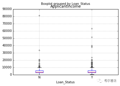
data.boxplot(column="ApplicantIncome",by="Loan_Status")

箱型图1

箱型图

因为之前没怎么接触过箱型图，所以这里单独开一节简单归纳一下。

箱形图（英文：Box-plot），又称为盒须图、盒式图、盒状图或箱线图，是一种用作显示一组数据分散情况资料的统计图。因型状如箱子而得名。详细解析看维基百科。

因为上面那幅图不太容易看，用个简单点的例子来说，还是上一小节那个只有a列和b列的表格。按b列对a列进行分组：

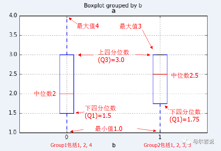
df_temp.boxplot(column="a",by="b")

箱型图2

定义b列值为0的分组为Group1，b列值为1的分组为Group2。Group1分组有4，2，1三个值，毫无疑问最大值4，最小值1，在箱型图中这两个值对应箱子发出的虚线顶端的两条实线。Group2分组有3，3，2，1四个值，由于最大值3和上四分位数3(箱子顶部)相同，所以重合了。

Group1中位数是2，而Group2的中位数则是中间两个数2和3的平均数，也即2.5。在箱型图中由箱子中间的有色线段表示。

四分位数

四分位数是统计学的一个概念。把所有数值由小到大排列好，然后分成四等份，处于三个分割点位置的数值就是四分位数，其中：

第一四分位数 (Q1)，又称“较小四分位数”或“下四分位数”，等于该样本中所有数值由小到大排列后，在四分之一位置的数。
第二四分位数 (Q2)，又称“中位数”，等于该样本中所有数值由小到大排列后，在二分之一位置的数。
第三四分位数 (Q3)，又称“较大四分位数”或“上四分位数”，等于该样本中所有数值由小到大排列后，在四分之三位置的数。

Notice：Q3与Q1的差距又称四分位距（InterQuartile Range, IQR）。

计算四分位数时首先计算位置，假设有n个数字，则：

Q1位置 = (n-1) / 4
Q2位置 = 2 * (n-1) / 4 = (n-1) / 2
Q3位置 = 3 * (n-1) / 4

如果n-1恰好是4的倍数，那么数列中对应位置的就是各个四分位数了。但是，如果n-1不是4的倍数呢？

这时位置会是一个带小数部分的数值，四分位数以距离该值最近的两个位置的加权平均值求出。其中，距离较近的数，权值为小数部分；而距离较远的数，权值为(1-小数部分)。

再看例子中的Group1，Q1位置为0.5，Q2位置为1，Q3位置为1.5。（注意：位置从下标0开始！），所以：

Q1 = 0.5*1+0.5*2 = 1.5
Q2 = 2
Q3 = 0.5*2+0.5*4 = 3

而Group2中，Q1位置为0.75，Q2位置为1.5，Q3位置为2.25。

Q1 = 0.25*1+0.72*2 = 1.75
Q2 = 0.5*2+0.5*3 = 2.5
Q3 = 0.25*3+0.75*3 = 3

这样是否就清晰多了XD 然而，四分位数的取法还存在分歧，定义不一，我在学习这篇文章时也曾经很迷茫，直到阅读了源码！！

因为Pandas库依赖numpy库，所以它计算四分位数的方式自然也是使用了numpy库的。而numpy中实现计算百分比数的函数为percentile，代码实现如下：

def percentile(N, percent, key=lambda x:x):
    """
    Find the percentile of a list of values.

    @parameter N - is a list of values. Note N MUST BE already sorted.
    @parameter percent - a float value from 0.0 to 1.0.
    @parameter key - optional key function to compute value from each element of N.

    @return - the percentile of the values
    """
    if not N:
        return None
    k = (len(N)-1) * percent
    f = math.floor(k)
    c = math.ceil(k)
    if f == c:
        return key(N[int(k)])
    d0 = key(N[int(f)]) * (c-k)
    d1 = key(N[int(c)]) * (k-f)
    return d0+d1

读一遍源码之后就更加清晰了。最后举个例子：

from numpy import percentile, mean, median
temp = [1,2,4] # 数列包含3个数
print(min(temp))
print(percentile(temp,25))
print(percentile(temp,50))
print(percentile(temp,75))
print(max(temp))

1
1.5
2.0
3.0
4

temp2 = [1,2,3,3


    
] # 数列包含4个数
print(min(temp2))
print(percentile(temp2,25))
print(percentile(temp2,50))
print(percentile(temp2,75))
print(max(temp2))

1
1.75
2.5
3.0
3

temp3 = [1,2,3,4,5] # 数列包含5个数
print(min(temp2))
print(percentile(temp3,25))
print(percentile(temp3,50))
print(percentile(temp3,75))
print(max(temp3))

1
2.0
3.0
4.0
5

不熟悉的话就再手撸一遍！！！不要怕麻烦！！！这一小节到此Over~

直方图

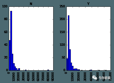
data.hist(column="ApplicantIncome",by="Loan_Status",bins=30)

直方图

直方图比箱型图熟悉一些，这里就不详细展开了。结合箱型图和直方图，我们可以看出获得贷款的人和未获得贷款的人没有明显的收入差异，也即收入不是决定性因素。

离群点

特别地，从直方图上我们可以看出这个数据集在收入字段上，比较集中于一个区间，区间外部有些散落的点，这些点我们称为离群点(Outlier)。前面将箱型图时没有细说，现在再回顾一下箱型图：

箱型图1

可以看到除了箱子以及最大最小值之外，还有很多横线，这些横线其实就表示离群点。那么可能又会有新的疑问了？怎么会有离群点在最大最小值外面呢？这样岂不是存在比最大值大，比最小值小的情况了吗？

其实之前提到一下，有一个概念叫四分位距（IQR），数值上等于Q3-Q1，记作ΔQ。定义：

最大值区间：Q3+1.5ΔQ
最小值区间：Q1-1.5ΔQ

也就是说最大值必须出现在这两个区间内，区间外的值被视为离群点，并显示在图上。这样做我们可以避免被过分偏离的数据点带偏，更准确地观测到数据的真实状况，或者说普遍状况。

想了解更多请阅读 Pandas Reference (hist) | Pandas Reference (boxplot)

10. 用Cut函数分箱

有时把数值聚集在一起更有意义。例如，如果我们要为交通状况（路上的汽车数量）根据时间（分钟数据）建模。具体的分钟可能不重要，而时段如“上午”“下午”“傍晚”“夜间”“深夜”更有利于预测。如此建模更直观，也能避免过度拟合。
这里我们定义一个简单的、可复用的函数，轻松为任意变量分箱。

#分箱:

def binning(col, cut_points, labels=None):

  #Define min and max values:

  minval = col.min()

  maxval = col.max()

  #利用最大值和最小值创建分箱点的列表

  break_points = [minval] + cut_points + [maxval]

  #如果没有标签，则使用默认标签0 ... (n-1)

  if not labels:

    labels = range(len(cut_points)+1)

  #使用pandas的cut功能分箱

  colBin = pd.cut(col,bins=break_points,labels=labels,include_lowest=True)

  return colBin



#为年龄分箱:

cut_points = [90,140,190]

labels = ["low","medium","high","very high"]

data["LoanAmount_Bin"] = binning(data["LoanAmount"], cut_points, labels)

print(pd.value_counts(data["LoanAmount_Bin"], sort=False))


low          104
medium       273
high         146
very high     91
dtype: int64

解析以下这段代码，首先定义了一个cut_points列表，里面的三个点用于把LoanAmount 字段分割成四个段，对应地，定义了labels列表，四个箱子(段)按贷款金额分别为低、中、高、非常高。然后把用于分箱的LoanAmount字段，cut_points，labels传入定义好的binning函数。

binning函数中，首先拿到分箱字段的最小值和最大值，把这两个点加入到break_points列表的一头一尾，这样用于切割的所有端点就准备好了。如果labels没有定义就默认按0~段数-1命名箱子。最后借助pandas提供的cut函数进行分箱。

cut函数原型是cut(x, bins, right=True, labels=None, retbins=False, precision=3, include_lowest=False)，x是分箱字段，bins是区间端点，right指示区间右端是否闭合，labels不解释..retbins表示是否需要返回bins，precision是label存储和显示的精度，include_lowest指示第一个区间的左端是否闭合。

在把返回的列加入到data后，使用value_counts函数，统计了该列的各个离散值出现的次数，并且指定不需要对结果进行排序。

想了解更多请阅读 Pandas Reference (cut)

11.为分类变量编码

有时，我们会面对要改动分类变量的情况。原因可能是：

有些算法（如logistic回归）要求所有输入项目是数字形式。所以分类变量常被编码为0, 1….(n-1)
有时同一个分类变量可能会有两种表现方式。如，温度可能被标记为“High”， “Medium”， “Low”，“H”， “low”。这里 “High” 和 “H”都代表同一类别。同理， “Low” 和“low”也是同一类别。但Python会把它们当作不同的类别。
一些类别的频数非常低，把它们归为一类是个好主意。

这里我们定义了一个函数，以字典的方式输入数值，用‘replace’函数进行编码

#使用Pandas replace函数定义新函数：

def coding(col, codeDict):

  colCoded = pd.Series(col, copy=True)

  for key, value in codeDict.items():

    colCoded.replace(key, value, inplace=True)

  return colCoded


#把贷款状态LoanStatus编码为Y=1, N=0:

print('Before Coding:')

print(pd.value_counts(data["Loan_Status"]))

data["Loan_Status_Coded"] = coding(data["Loan_Status"], {'N':0,'Y':1})

print('\nAfter Coding:')

print(pd.value_counts(data["Loan_Status_Coded"]))


Before Coding:
Y    422
N    192
Name: Loan_Status, dtype: int64

After Coding:
1    422
0    192
Name: Loan_Status_Coded, dtype: int64

在coding函数中第二个参数是一个dict，定义了需要编码的字段中每个值对应的编码。
实现上首先把传入的列转换为Series对象，copy参数表示是否要进行复制，关于copy可以看我另一篇笔记：深拷贝与浅拷贝的区别。

copy得到的Series对象不会影响到原本DataFrame传入的列，所以可以放心修改，这里replace函数中的inplace参数表示是否直接在调用对象上作出更改，我们选择是，那么colCoded对像在调用replace后就会被修改为编码形式了。最后，把编码后的列加入到data中，比较编码前后的效果。

想了解更多请阅读 Pandas Reference (replace)

12. 在一个数据框的各行循环迭代

有时我们会需要用一个for循环来处理每行。比方说下面两种情况：

带数字的分类变量被当做数值。
带文字的数值变量被当做分类变量。

先看看data表格的数据类型：

#检查当前数据类型：

data.dtypes

结果：

Gender                 object
Married                object
Dependents             object
Education              object
Self_Employed          object
ApplicantIncome         int64
CoapplicantIncome     float64
LoanAmount            float64
Loan_Amount_Term      float64
Credit_History        float64
Property_Area          object
Loan_Status            object
LoanAmount_Bin       category
Loan_Status_Coded       int64
dtype: object

可以看到Credit_History这一列被当作浮点数，而实际上我们原意是分类变量。所以通常来说手动定义变量类型是个好主意。那这种情况下该怎么办呢？这时我们需要逐行迭代了。

首先创建一个包含变量名和类型的csv文件，读取该文件：

#载入文件:
colTypes = pd.read_csv(r'F:\Datahack_Loan_Prediction\datatypes.csv')
print(colTypes)

              feature         type
0             Loan_ID  categorical
1              Gender  categorical
2             Married  categorical
3          Dependents  categorical
4           Education  categorical
5       Self_Employed  categorical
6     ApplicantIncome   continuous
7   CoapplicantIncome   continuous



    
8          LoanAmount   continuous
9    Loan_Amount_Term   continuous
10     Credit_History  categorical
11      Property_Area  categorical
12        Loan_Status  categorical

载入这个文件之后，我们能对它的逐行迭代，然后使用astype函数来设置表格的类型。这里把离散值字段都设置为categorical类型(对应np.object)，连续值字段都设置为continuous类型（对应np.float）。

#迭代每行，指派变量类型。

#注，astype函数用于指定变量类型。

for i, row in colTypes.iterrows(): #i: dataframe索引; row: 连续的每行

    if row['type']=="categorical" and row['feature']!="Loan_ID":
        data[row['feature']]=data[row['feature']].astype(np.object)
    elif row['type']=="continuous":
        data[row['feature']]=data[row['feature']].astype(np.float)

print(data.dtypes)

Gender                object
Married               object
Dependents            object
Education             object
Self_Employed         object
ApplicantIncome      float64
CoapplicantIncome    float64
LoanAmount           float64
Loan_Amount_Term     float64
Credit_History        object
Property_Area         object
Loan_Status           object
dtype: object

可以看到现在信用记录(Credit_History)这一列的类型已经变成了‘object’ ，这在Pandas中代表分类变量。

特别地，无论是中文教程还是原版英文教程这个地方都出错了.. 中文教材代码中判断条件是错的，英文教程中没有考虑到Loan_ID这个字段，由于它被设定为表格的索引，所以它的类型是不被考虑的。

想了解更多请阅读 Pandas Reference (iterrows)

手把手教你学python第三课：数据分析，学会使用​pandas大杀器