👇点击关注公众号👇
第一时间获取人工智能干货内容
本文,我们通过Python实现回归分析。
首先导入相关的包,读取相关数据:
import pandas as pd
f = open('D:/机器学习数据/salary.csv')
df = pd.read_csv(f, index_col = 0)
df.head()
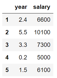
研究工作年限与薪资情况
导入绘图模块,取出需要的数据:
from matplotlib import pyplot as plt
X = df[['year']]
Y = df['salary'].values#从array取出数据
查看数据前五行:
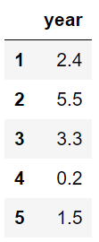
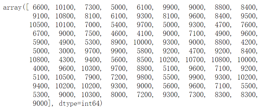
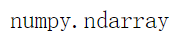
Y的数据类型是numpy的n维数组类型。
接下来进行一元线性回归
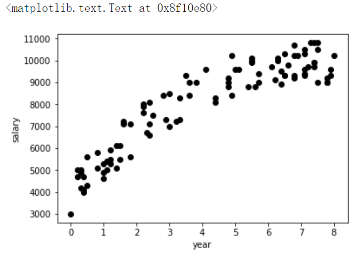
绘制散点图:
% matplotlib inline
plt.scatter(X,Y, color="black")#绘制散点图
plt.xlabel('year')#x轴标签
plt.ylabel('salary')#y轴标签
导入线性回归模块,训练模型:
from sklearn.linear_model import LinearRegression
regr = LinearRegression()#创建一个线性回归对象
regr.fit(X,Y)#线性回归拟合数据

输出截距和系数值:
print('Coefficient:{}'.format(regr.coef_) )#系数K
print('Intercept:{}'.format(regr.intercept_) )#截距

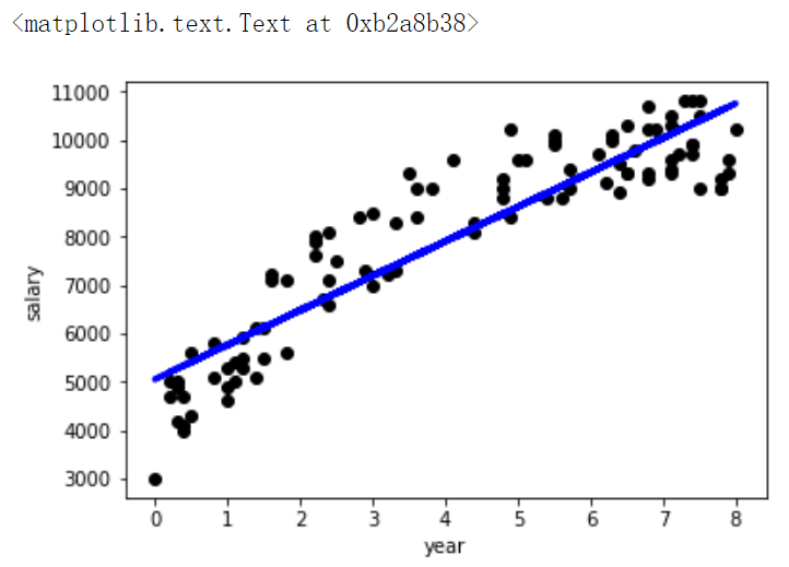
绘制回归结果:
plt.scatter(X,Y, color="black")
plt.plot(X, regr.predict(X), linewidth = 3, color = "blue")#画出回归线
plt.xlabel('year')
plt.ylabel('salary')
接下来进行多项式线性回归:
from sklearn.preprocessing import PolynomialFeatures
from sklearn.linear_model import LinearRegression#多项式线性回归

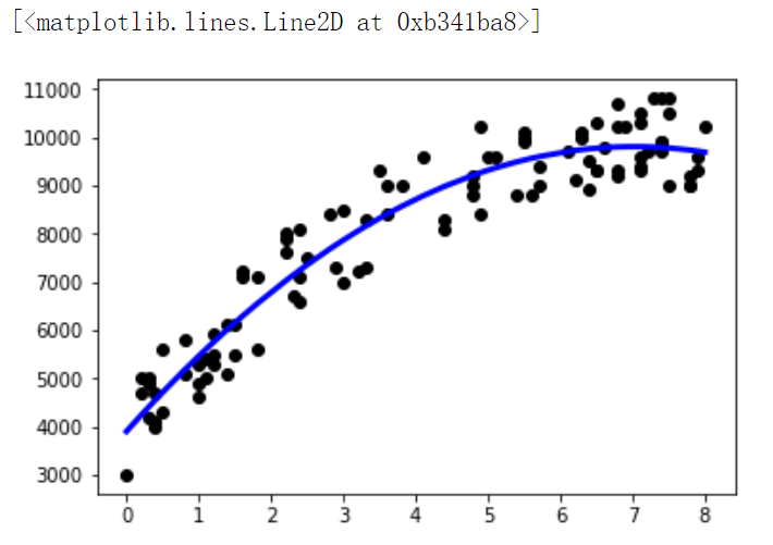
poly_reg= PolynomialFeatures(degree = 2)#二次项
X_ = poly_reg.fit_transform(X)
regr = LinearRegression()
regr.fit(X_, Y)

转换数据类型:
X2 = X.sort_values(['year'])#x排序,根据year排序
X2_ = poly_reg.fit_transform(X2)#dataframe转换为ndarray
绘图:
plt.scatter(X,Y, color="black")
plt.plot(X2, regr.predict(X2_), color= "blue", linewidth = 3)
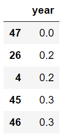
查看数据前五行:
查看数据类型:

接下来看看多元回归分析房屋价格影响因素
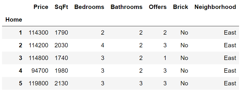
导入数据:
import pandas
f = open('D:/机器学习数据/house-prices.csv')
df = pd.read_csv(f, index_col = 0)

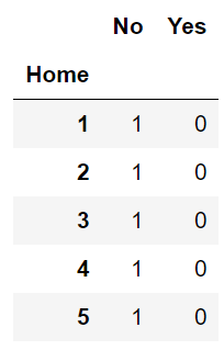
对变量做虚拟变量化:
pandas.get_dummies(df['Brick']).head()
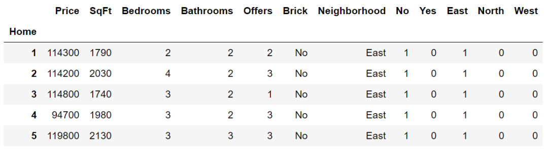
对数据做拼接:
house = pandas.concat([df, pandas.get_dummies(df['Brick']), pandas.get_dummies(df['Neighborhood'])], axis = 1)#合并
house.head()
删除多余的东西:
#去除多余的内容
del house['No']
del house['West']
del house['Brick']
del house['Neighborhood']
#del house['Home']
house.head()
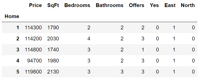
查看列:

X = house[['SqFt', 'Bedrooms', 'Bathrooms', 'Offers', 'Yes', 'East', 'North']]#选取自变量
Y = house['Price'].values#因变量
搭建回归模型:
#建立多元线性回归模型
from sklearn.linear_model import LinearRegression
regr = LinearRegression()
regr.fit(X,Y)

预测:
#regr.predict(X)
X1 = [[1000, 2 , 1, 1, 1, 0 ,0]] #预测
regr.predict(X1)

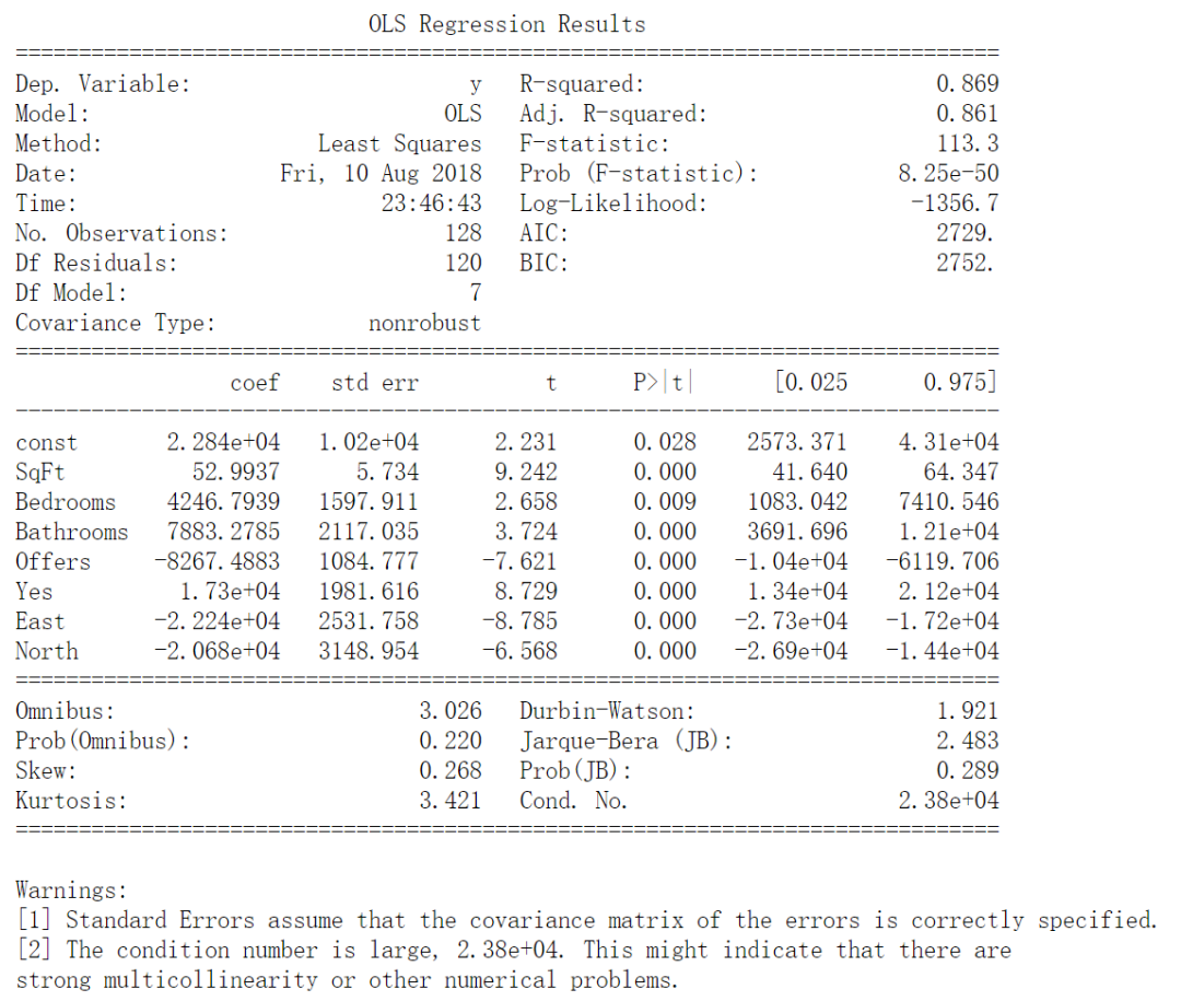
计算统计相关参数:
import statsmodels.api as sm
X2 = sm.add_constant(X)
est = sm.OLS(Y, X2)
est2 = est.fit()
print(est2.summary())

#coef   相关系数
选择最佳参数:
#选择最佳参数组合
predictorcols = [ 'SqFt', 'Bedrooms', 'Bathrooms', 'Offers', 'Yes', 'East', 'North']

import itertools
AICs = {}
for k in range(1,len(predictorcols)+1):#多种个数情况都考虑
    for variables in itertools.combinations(predictorcols, k):
        predictors  = X[list(variables)]
        predictors2 = sm.add_constant(predictors)
        est = sm.OLS(Y, predictors2)
        res = est.fit()
        AICs[variables] = res.aic#组合与AIC值
统计最佳组合:
from collections import Counter
c = Counter(AICs)#Count可以计数
#c.most_common()#列出最高的
c.most_common()[::-10]#最佳组合排名
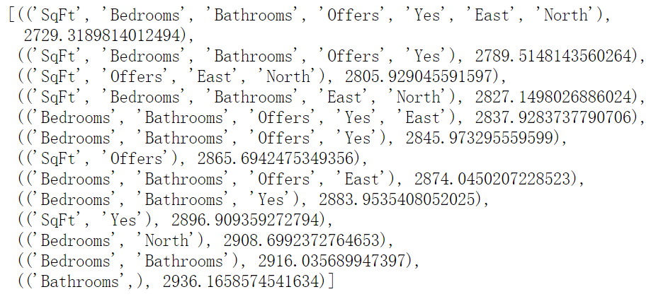
选择AIC较小的作为模型参数。
这就是本篇回归分析的实战内容了!你学会了么?