本文通过Python代码实现PCA降维。
先贴代码,再讲解:
# 导入pandas用于数据读取和处理。
import pandas as pd
import numpy as np
%matplotlib inline
# 从互联网读入手写体图片识别任务的训练数据,存储在变量digits_train中。
digits_train = pd.read_csv('https://archive.ics.uci.edu/ml/machine-learning-databases/optdigits/optdigits.tra', header=None)
# 从互联网读入手写体图片识别任务的测试数据,存储在变量digits_test中。
digits_test = pd.read_csv('https://archive.ics.uci.edu/ml/machine-learning-databases/optdigits/optdigits.tes', header=None)
# 分割训练数据的特征向量和标记。
X_digits = digits_train[np.arange(64)]#64维度
y_digits = digits_train[64]#第65维:数字类别
# 从sklearn.decomposition导入PCA。
from sklearn.decomposition import PCA
# 初始化一个可以将高维度特征向量(64维)压缩至2个维度的PCA。
estimator = PCA(n_components=2)
X_pca = estimator.fit_transform(X_digits)
# 显示10类手写体数字图片经PCA压缩后的2维空间分布。
from matplotlib import pyplot as plt
def plot_pca_scatter():
colors = ['black', 'blue', 'purple', 'yellow', 'white', 'red', 'lime', 'cyan', 'orange', 'gray']#10类的颜色设置
for i in range(len(colors)):#10类从0~9循环
px = X_pca[:, 0][y_digits.as_matrix() == i]#如果属于第i类,x维度
py = X_pca[:, 1][y_digits.as_matrix()== i]
plt.scatter(px, py, c=colors[i])#画散点图
plt.legend(np.arange(0,10).astype(str))#图例是0~9数字
plt.xlabel('First Principal Component'
)#第一主成分
plt.ylabel('Second Principal Component')#第二主成分
plt.show()
plot_pca_scatter()
以上代码,首先导入需要的包,然后读取数据(需要联网导入数据)。
之后将数据的特征和标签进行分割保存。
之后导入PCA模块。
以上代码中已经加入详细注释,相信大家容易理解。
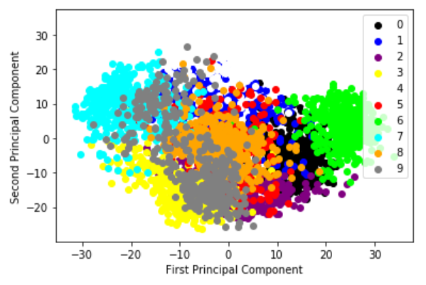
将原始的64维数据压缩至2维,并且可视化,结果如下:
查看训练集标签的数据情况:
array([0, 0, 7, ..., 6, 6, 7], dtype=int64)
查看训练集特征的数据量:
3823
查看属于第一类的数据条数:
len(X_pca[:, 0][y_digits.as_matrix() == 1])
389
接下来使用原始像素特征和经PCA压缩重建的低维特征,在相同配置的支持向量机分类模型上分别进行图像识别。
代码如下:
# 对训练数据、测试数据进行特征向量(图片像素)与分类目标的分隔。
X_train = digits_train[np.arange(64)]
y_train = digits_train[64]
X_test = digits_test[np.arange(64)]
y_test = digits_test[64]

# 导入基于线性核的支持向量机分类器。
from sklearn.svm import LinearSVC

# 使用默认配置初始化LinearSVC,对原始64维像素特征的训练数据进行建模,并在测试数据上做出预测,存储在y_predict中。
svc = LinearSVC()
svc.fit(X_train, y_train)
y_predict = svc.predict(X_test)

# 使用PCA将原64维的图像数据压缩到20个维度。
estimator = PCA(n_components=20)

# 利用训练特征决定(fit)20个正交维度的方向,并转化(transform)原训练特征。
pca_X_train = estimator.fit_transform(X_train)
# 测试特征也按照上述的20个正交维度方向进行转化(transform)。
pca_X_test = estimator.transform(X_test)

# 使用默认配置初始化LinearSVC,对压缩过后的20维特征的训练数据进行建模,并在测试数据上做出预测,存储在pca_y_predict中。
pca_svc = LinearSVC()
pca_svc.fit(pca_X_train, y_train)
pca_y_predict = pca_svc.predict(pca_X_test)
以上分别使用压缩前后建模,具体注释写了很多,相信大家能看懂。
接下来是对比压缩前后模型评估效果。
# 从sklearn.metrics导入classification_report用于更加细致的分类性能分析。
from sklearn.metrics import classification_report
# 对使用原始图像高维像素特征训练的支持向量机分类器的性能作出评估。
print(svc.score(X_test, y_test))
print(classification_report(y_test, y_predict, target_names=np.arange(10).astype(str)))
# 对使用PCA压缩重建的低维图像特征训练的支持向量机分类器的性能作出评估。
print(pca_svc.score(pca_X_test, y_test))
print(classification_report(y_test, pca_y_predict, target_names=np.arange(10).astype(str)))
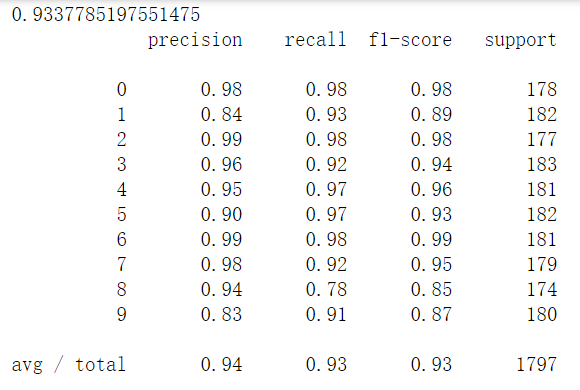
压缩前的模型评估结果:
压缩后的模型评估结果:
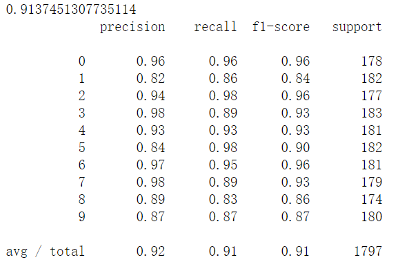
通过对比结果发现,经过PCA特征压缩和重建之后的特征数据会损失2%左右的预测准确性,但是相比于原始数据64维度的特征而言,我们使用PCA降低了很多维度!大大减少了数据运算量。
这就是Python的PCA降维实战部分,你学会了么?