一:综述
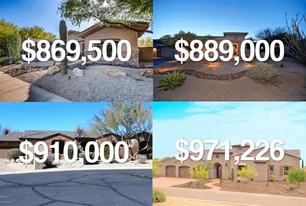
今天为大家介绍一个用Keras神经网络构建回归模型以预测房价的案例。
 img
img这个案例中依赖的库有
 img
img数据集来自 https://github.com/emanhamed/Houses-dataset。该数据集包括csv文件以及图像。本文主要利用该数据集的csv文件部分来训练模型。
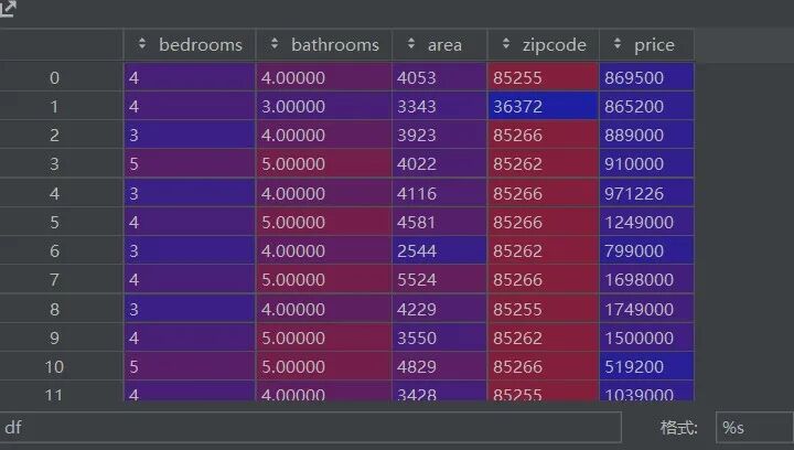
我们先来看看数据集的样子
cols = ["bedrooms", "bathrooms", "area", "zipcode", "price"]
import pandas as pd
df = pd.read_csv("E:\code\RegressionWithKeras\RegressionWithKeras\HousesDataset\HousesDataset\HousesInfo.txt", sep=" ", header=None, names=cols)
 img
img包含五个列:房间数、浴室数、面积、邮政编码以及价格,其中价格是我们的目标列,其它则作为特征列。
二:数据清洗
在这个数据集中,有一些邮政编码对应的数据很少,是数据集的”噪声“,应该被去除。所以,编写一个函数,用以清洗数据集,代码如下:
def load_house_attributes(inputPath):
    # 加载数据集
    cols = ["bedrooms", "bathrooms", "area", "zipcode", "price"]
    df = pd.read_csv(inputPath, sep=" ", header=None, names=cols)
    # zipcodes是每个邮政编码的值
    # counts则是每个邮政编码出现的次数
    zipcodes = df["zipcode"].value_counts().keys().tolist()
    counts = df["zipcode"].value_counts().tolist()
    # 遍历它们的组合,找出小于阈值25的编码,把它们从df中删掉
    for (zipcode, count) in zip(zipcodes, counts):
        if count 25:
            idxs = df[df["zipcode"] == zipcode].index
            df.drop(idxs, inplace=True)
    return df
这个函数接受数据集路径,统计数据集中邮政编码的出现次数,剔除出现次数小于25的数据,返回清洗后的dataframe,调用此函数
# 设置数据集的路径,加载数据集
print("[INFO] loading house attributes...")
inputPath = "./HousesDataset/HousesDataset/HousesInfo.txt"
df = datasets.load_house_attributes(inputPath)
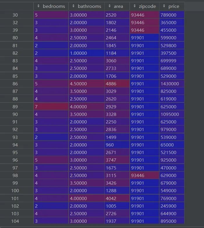
清洗后的数据如下所示:
 img
img可以看出,清洗后的数据index从30开始,剔除了一些数据。
清洗完成后,我们来划分训练集和测试集,借助sklearn,很容易完成。
print("[INFO] constructing training/testing split...")
(train, test) = train_test_split(df, test_size=0.25, random_state=42)
三:特征工程
现在让我们把一些连续的数值特征作归一化处理,包括房间数、浴室数和面积,归一化处理能让我们训练的收敛速度更快。
连续特征处理完了,分类属性也要处理,一般我们就用one—hot编码对离散特征进行处理
同样构造一个函数来完成。代码如下:
def process_house_attributes(df, train, test):
    # 要处理的连续特征
    continuous = ["bedrooms", "bathrooms", "area"]
    # 通过MinMax转换器,把它们都变成0~1之间的数
    cs = MinMaxScaler()
    trainContinuous = cs.fit_transform(train[continuous])
    testContinuous = cs.transform(test[continuous])
    # 通过LabelBinarizer转换器,将邮政编码进行one-hot编码
    zipBinarizer = LabelBinarizer().fit(df["zipcode"])
    trainCategorical = zipBinarizer.transform(train["zipcode"])
    testCategorical = zipBinarizer.transform(test["zipcode"])
    # 将处理后的特征拼接起来,构成训练集
    trainX = np.hstack([trainCategorical, trainContinuous])
    testX = np.hstack([testCategorical, testContinuous])
    # return the concatenated training and testing data
    return (trainX, testX)
这个函数接收清洗后的dataframe以及划分好的训练集,测试集,通过对连续属性进行归一化、离散属性one-hot化,对特征进行进一步处理,最后返回训练特征数据集和测试特征数据集(相比原来剔除了目标列)。
# 对特征列进行归一化和one—hot编码
print("[INFO] processing data...")
(trainX, testX) = datasets.process_house_attributes(df, train, test)
因为目标列也是连续属性,所以也进行归一化处理
# 对目标列也进行归一化
maxPriceTrain = train["price"].max()
maxPriceTest = test["price"].max()
trainY = train["price"] / maxPriceTrain
testY = test["price"] / maxPriceTrain
四:模型建立
使用Keras构建多层感知机模型,也叫人工神经网络ANN。MLP适用于分类预测问题,输入一组数据,输出一个分类。它们也适用于回归预测问题,输入一组数据,输出一个连续值。
如图所示:
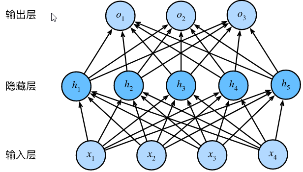 img
img代码如下:
def create_mlp(dim, regress=False):
# 定义MLP神经网络
model = Sequential()
# 在网络上加两个层,一层节点为8,另一层节点为4,两层的激活函数都是relu
model.add(Dense(8, input_dim=dim, activation="relu"))
model.add(Dense(4, activation="relu"))
# 如果用于回归任务,再加一层(输出层),激活函数为linear
if regress:
model.add(Dense(1, activation="linear"))
# 返回model
return model
# 构建MLP模型
model = models.create_mlp(trainX.shape[1], regress=True)
# 其中opt包含了lr学习率,以及decay衰减率
opt = Adam(lr=1e-3, decay=1e-3 / 200)
# 设置损失函数为MAPE,并且传入opt,完成模型的构建
model.compile(loss=
"mean_absolute_percentage_error", optimizer=opt)
五:训练模型并预测
# 训练模型,训练2000轮,每一轮的用8个样本更新梯度(小批量梯度下降算法)
print("[INFO] training model...")
model.fit(x=trainX, y=trainY,
validation_data=(testX, testY),
epochs=2000, batch_size=8)
# 在测试集上作预测
print("[INFO] predicting house prices...")
preds = model.predict(testX)
# 计算误差、误差百分比、误差百分比的绝对值
diff = preds.flatten() - testY
percentDiff = (diff / testY) * 100
absPercentDiff = np.abs(percentDiff)
# 对误差百分比的绝对值求均值和标准差
mean = np.mean(absPercentDiff)
std = np.std(absPercentDiff)
# 打印模型训练的相关指标
locale.setlocale(locale.LC_ALL, "en_US.UTF-8")
print("[INFO] avg. house price: {}, std house price: {}".format(
locale.currency(df["price"].mean(), grouping=True),
locale.currency(df["price"].std(), grouping=True)))
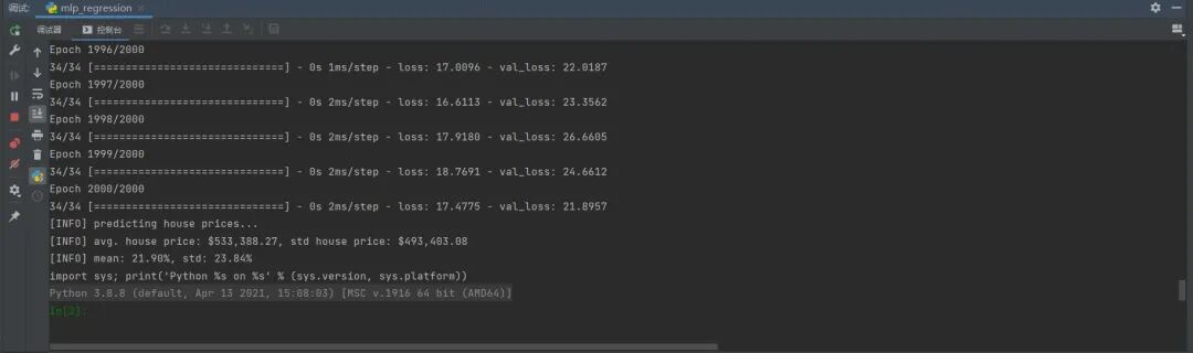
print("[INFO] mean: {:.2f}%, std: {:.2f}%".format(mean, std))
运行结果如下:
 img
img六:进一步学习
对MLP不熟悉的朋友们可以看B站UP主 3blue1Brown 出品的深度神经网络视频。
关于Keras的更多知识以及api使用可以访问它的中文文档进行进一步的学习:https://keras.io/zh/
最后,推荐蚂蚁老师的Python全栈课程: