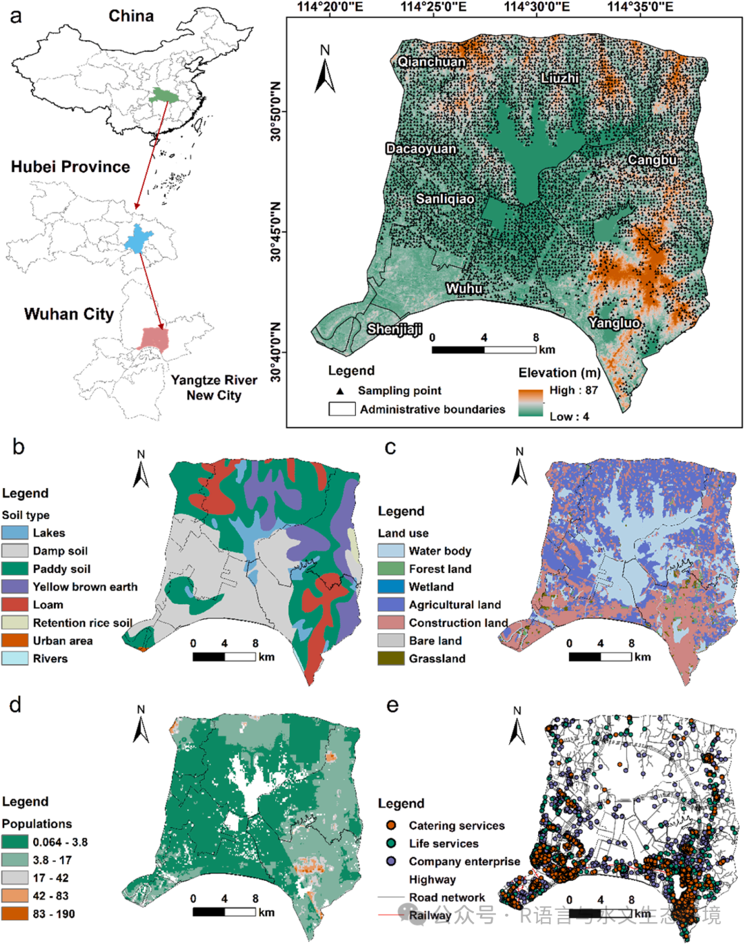
Fig. 1. Overview of the study area. (a) Map of the study location and soil sampling points; (b) Soil type distribution; (c) Land use patterns; (d) Population density; (e) Distribution of domestic services, businesses, and restaurants.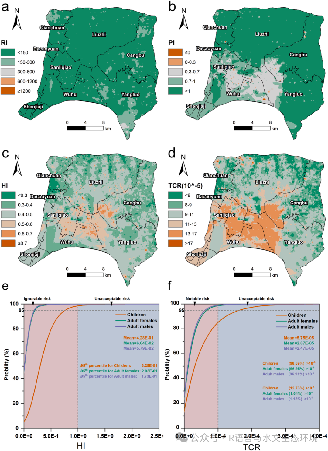
Fig. 2. Pollution risk of soil HMs. (a) Potential ecological risks; (b) Environmental capacity risk; (c) Non-carcinogenic risks; (d) Carcinogenic risks; (e) Probability
distribution of non-carcinogenic risk; (f) Carcinogenic risk probability distribution.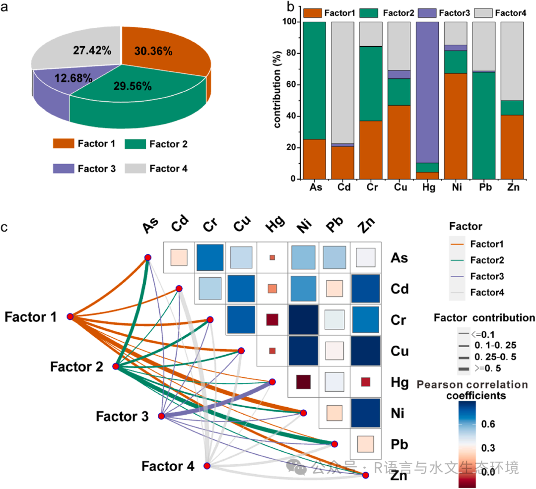
Fig. 3. Analysis of sources contributing to soil HMs contamination. (a) The PMF model was used to estimate the percentage contribution of each source. (b) The PMF model also revealed the contribution and distribution of four factors across the HMs. (c) The correlation between HMs was assessed by integrating Pearson correlation analysis with the PMF model. 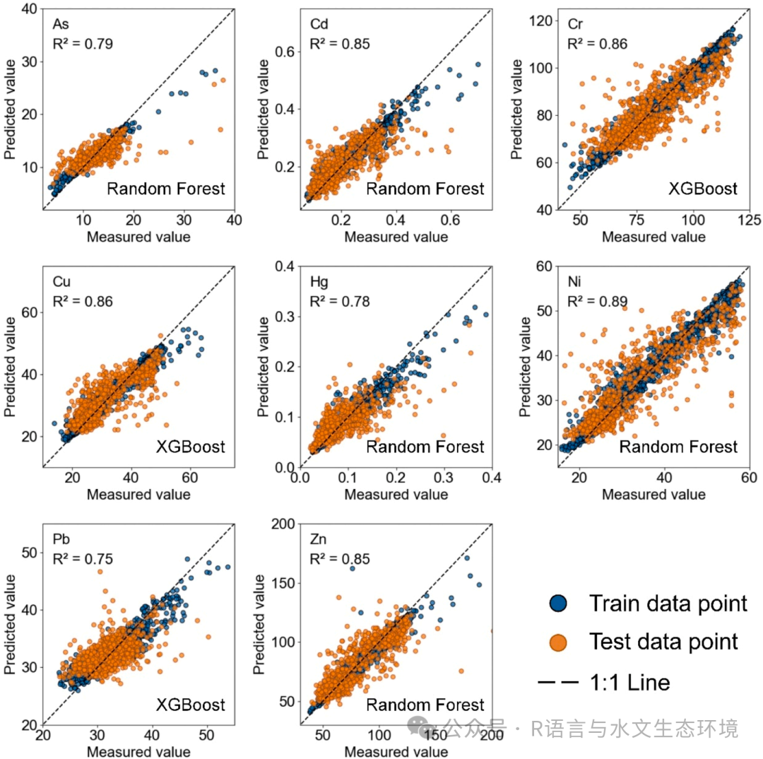
Fig. 4. Scatter plots of measured versus predicted concentrations for the train and test data were generated using the RF and XGB models for soil HMs. Blue dots represent the training data, while orange dots represent the test data. The gray dashed line indicates the 1:1 line, representing agreement between measured and predicted values.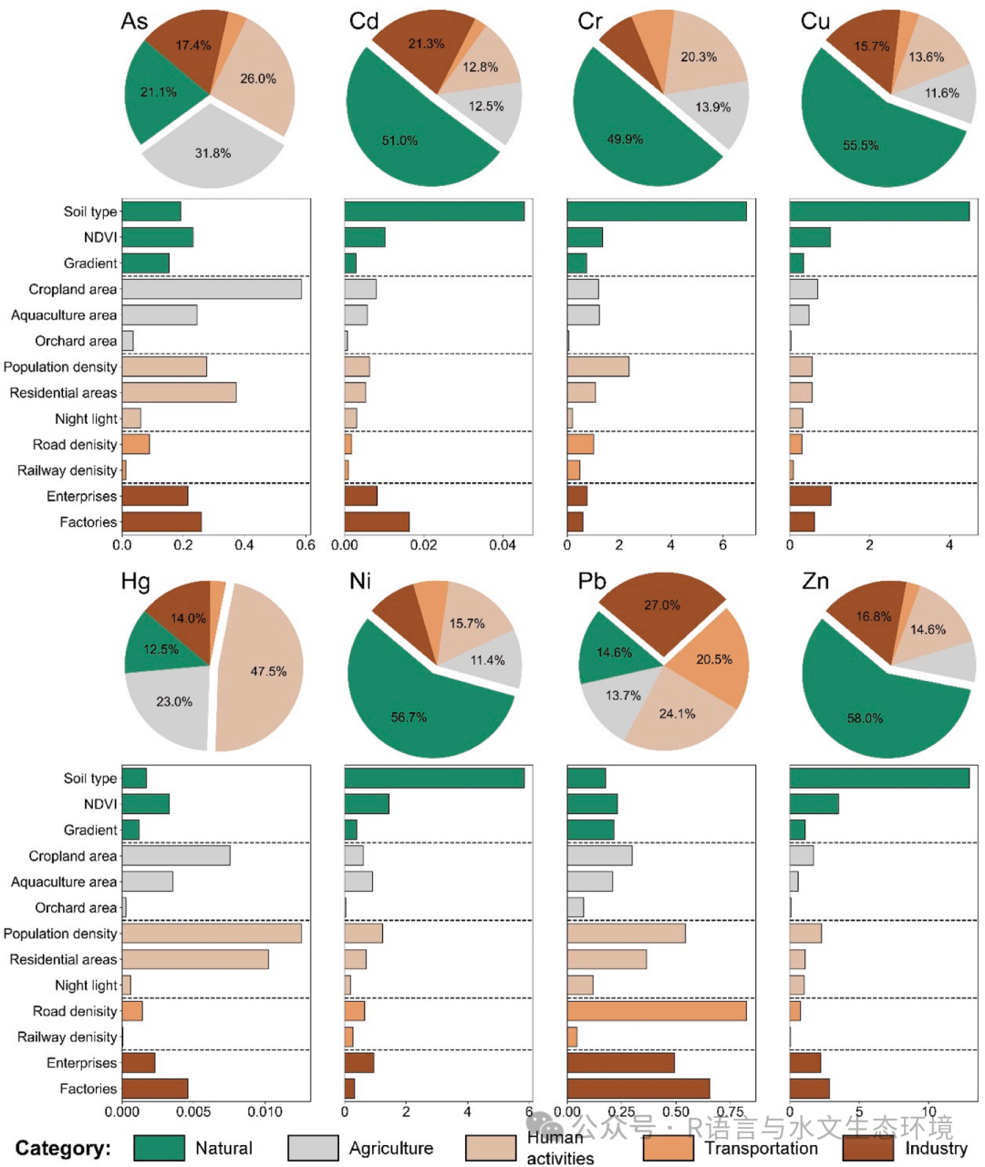
Fig. 5. Importance analysis of environmental and socio-economic variables on soil HMs contamination.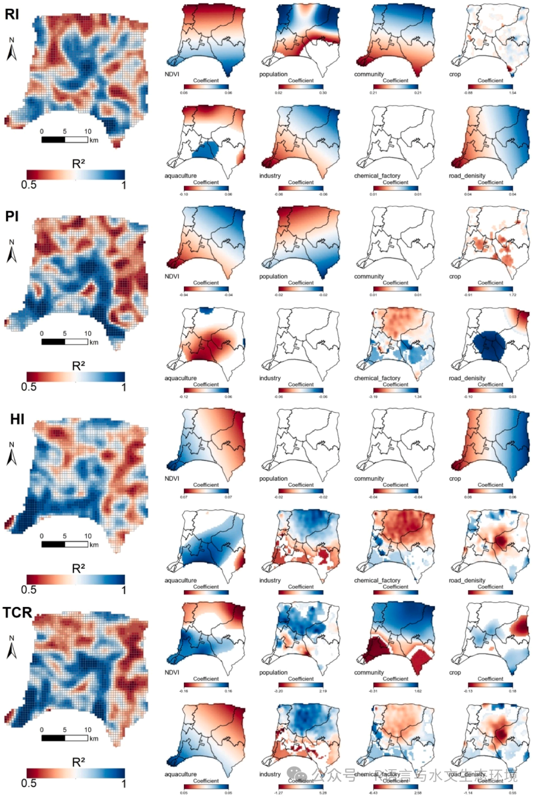
Fig. 6. Spatial distribution of key influencing factors for pollution risks (RI, PI, HI, TCR) using the MGWR model. The blank grid cell areas indicate non-significant regression results (p > 0.05).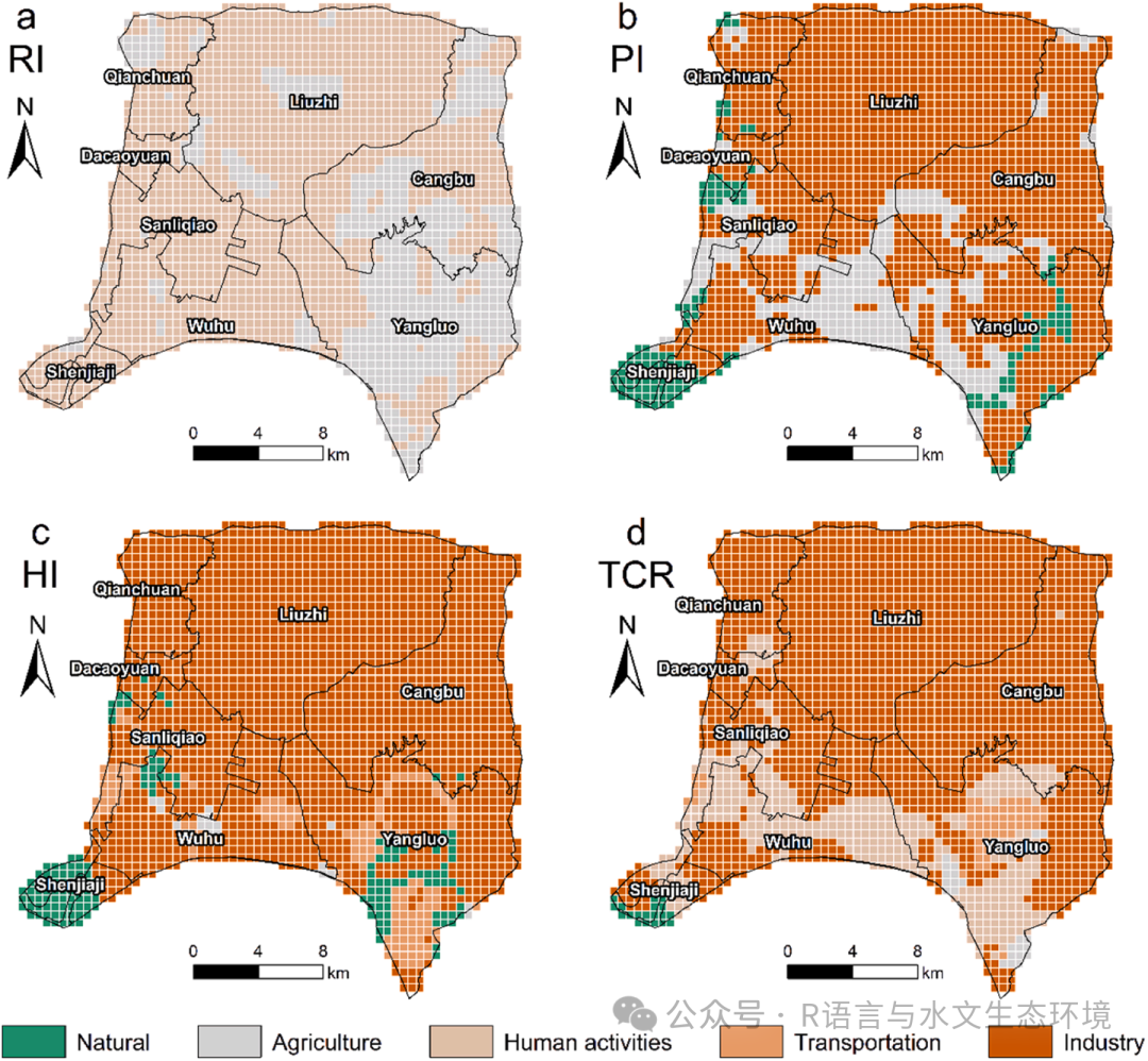
Fig. 7. Spatial distribution of major contributing pollution source categories for soil HMs risks in the study area. |