Fig. 1.Steps in estimating groundwater head and surface water depth: (A) hydrological simulation using the physics-based model HGS, (B–C) preparation of the DL dataset, (D) configuration of the DL model, (E) optimization of input data and the DL model, (F) estimation of groundwater and surface water conditions using the optimal DL model, and (G) prediction of future hydrological responses under climate change scenarios. In (D), the colored rectangular blocks represent multiple layers comprising a CNN structure (for example, convolutional, pooling, ReLU, and normalization layers). Detailed information on these layers can be found in the Supplementary Information (Appendix B.2). 
Fig. 2.Spatiotemporal maps of estimated groundwater heads using the optimal DL model (A), HGS model (B), and their prediction discrepancy (C). Subplots 1–4 present mapping results for March, June, September, and December 2016, respectively. (Mapping results for other periods can be found in a supplementary video clip). In panels (A) and (B), the color bar indicates groundwater head (m), with red representing higher values and blue representing lower values. In panel (C), the color bar displays the estimation discrepancy between the HGS and optimal DL models (i.e., ground-truth - DL prediction), with red indicating underestimations and blue indicating overestimations of the DL model compared to the HGS model. 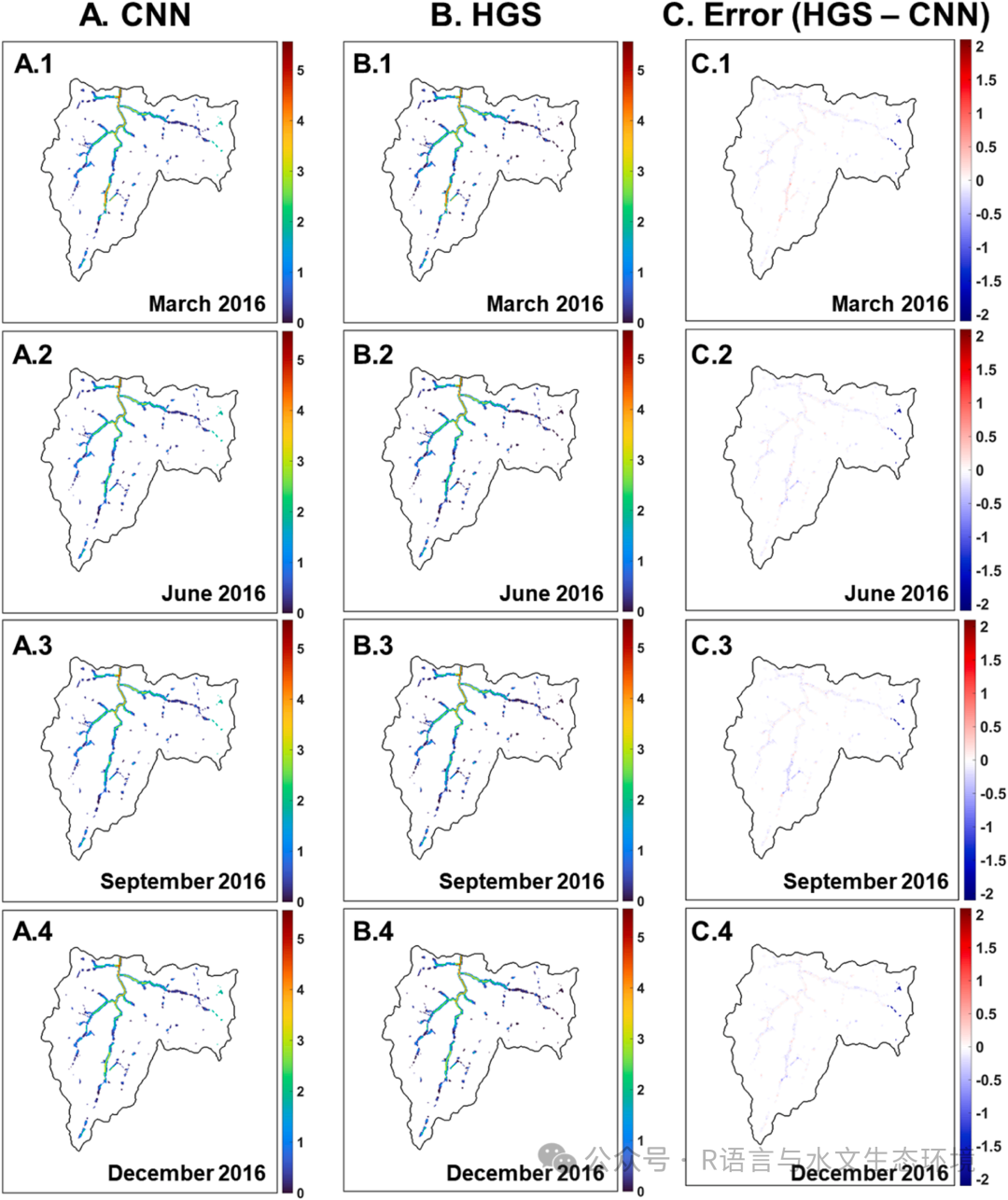 Fig. 3.Spatiotemporal maps of estimated surface water depths using the optimal DL model (A), HGS model (B), and their prediction discrepancy (C). Subplots 1–4present mapping results for March, June, September, and December 2016, respectively, while mapping results for other periods can be found in a supplementary video clip. In panels (A) and (B), the color bar indicates surface water depth (m), with red representing higher values and blue representing lower values. In panel (C),the color bar displays the estimation discrepancy between the HGS and optimal DL models (i.e., ground-truth - DL prediction), with red indicating underestimations and blue indicating overestimations of the DL model compared to the HGS model. 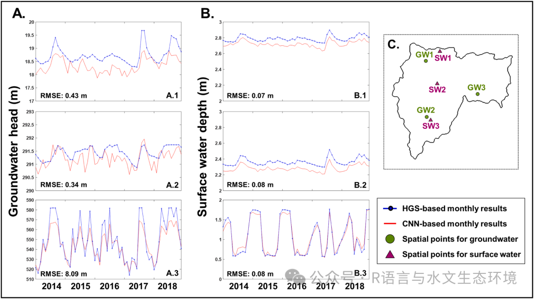 Fig. 4.Time-series plots of estimated groundwater head (A) and surface water depth (B). Hydrological conditions from 2014 to 2018 were collected at spatial points (C). The blue dotted line indicates the HGS model, while the red line represents the optimal CNN model. Light green circles indicate spatial points for groundwater (GW1–3), while fuchsia triangles indicate spatial points for surface water (SW1–3). Subplots A.1–3 correspond to the results at GW1–3, respectively, and subplots B.1–3 represent the results at SW1–3, respectively |


 关注我们
关注我们