逻辑回归是继线性回归之后最著名的机器学习算法。

在很多方面，线性回归和逻辑回归是相似的，不过最大的区别在于它们的用途，线性回归算法用于预测，但逻辑回归用于分类任务。

分类任务很常见，比如把电子邮件分为垃圾邮件和非垃圾邮件、把肿瘤分为恶性或者良性、把网站分为危险站点或正常站点，机器学习算法就可以完成这些任务。

其中，逻辑回归算法就是一种分类算法，简单粗暴，但有用。



现在，开始深入研究逻辑回归。

Sigmoid函数（Logistic函数）

逻辑回归算法使用具有独立预测因子的线性方程来预测，预测值可以是从负无穷到正无穷之间的任何值。

我们需要让算法的输出为类变量，比如用0表示非，用1表示是。

因此，我们将线性方程的输出压缩到[0,1]的范围内。

为了压缩0和1之间的预测值，我们使用sigmoid函数：

△ 线性方程和sigmoid函数

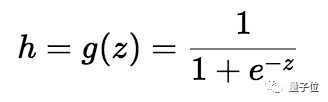
△ 压缩输出-h

我们取线性方程的输出（z）并给出返回压缩值h的函数g（x），h将位于0到1的范围内。为了理解sigmoid函数如何压缩，我们画出了sigmoid函数的图形：

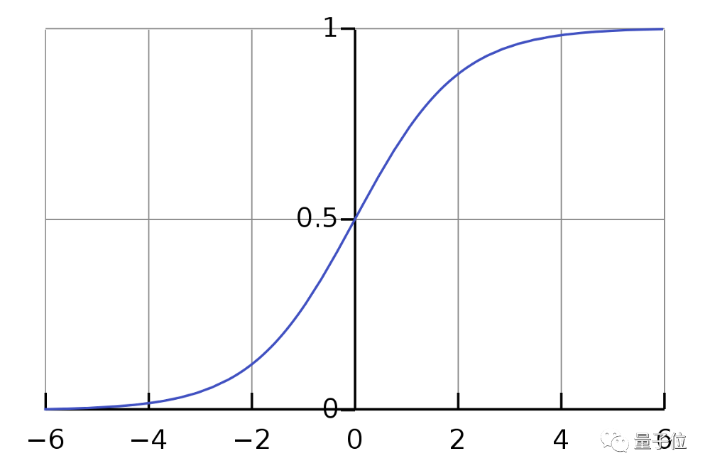
△ sigmoid函数图形

如图可见，sigmoid函数当x>0时，y逐渐向1靠近；当x<0时，y逐渐向0靠近。

成本函数（cost function）

由于我们试图预测类别值，不能使用和线性回归算法中相同的成本函数。

所以，我们使用损失函数的对数来计算错误分类的成本。

考虑到计算上面这个函数的梯度实在太难了，，我们把它写成下面这个样子：

计算梯度

我们取相对于每个参数（θ_0，θ_1，…）的成本函数的偏导数来获得梯度，有了这些梯度，我们可以更新θ_0，θ_1，…的值。

现在，开始召唤微积分大法：

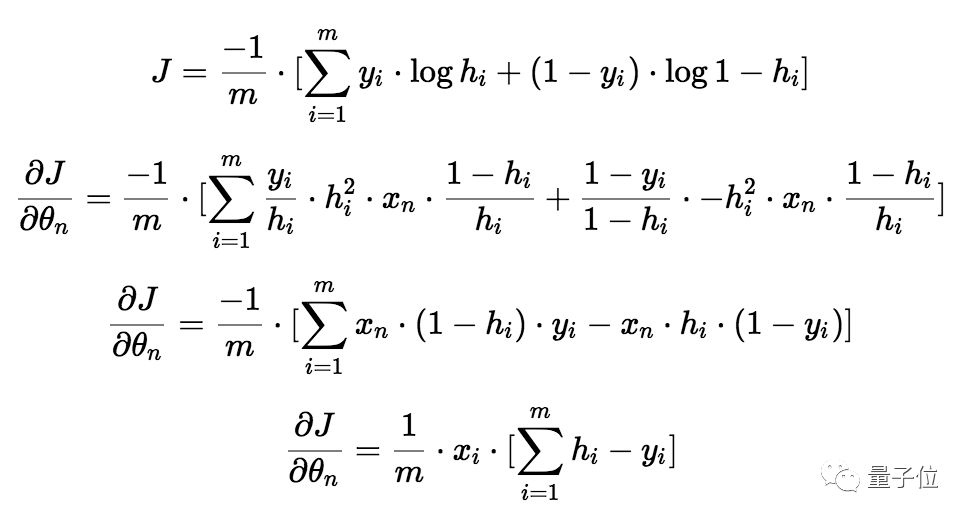
△ 梯度

如果看懂了，那你的微积分学得棒棒的。



不过，如果微积分大法召唤失败……就直接照着上面的式子做吧。

写代码

现在方程终于搞定了，开始写代码。

我们用NumPy来从头构建模型，用IRIS（鸢尾花）数据集来训练和测试算法。

 1import pandas as pd
 2
 3df = pd.read_csv('/Users/rohith/Documents/Datasets/Iris_dataset/iris.csv') ## Load data
 4df = df.drop(['Id'],axis=1)
 5rows = list(range(100,150))
 6df = df.drop(df.index[rows])  ## Drop the rows with target values Iris-virginica
 7Y = []
 8target = df['Species']
 9for val in target:
10    if(val == 'Iris-setosa'):
11        Y.append(0)
12    else:
13        Y.append(1)



    
14df = df.drop(['Species'],axis=1)
15X = df.values.tolist()

我们用pandas来加载数据。

IRIS数据集有三个目标值，分别是弗吉尼亚鸢尾、山鸢尾、变色鸢尾。但是因为要实现的是二进制的分类算法，所以此处先把弗吉尼亚鸢尾剔除。

△ 变色鸢尾（左）和山鸢尾（右），图源百度百科

现在，只剩下两个目标值用来分类了。

之后，从数据集中提取独立变量和因变量，现在可以继续准备训练集和测试集了。

 1from sklearn.utils import shuffle
 2from sklearn.cross_validation import train_test_split
 3import numpy as np
 4
 5X, Y = shuffle(X,Y)
 6
 7x_train = []
 8y_train = []
 9x_test = []



    
10y_test = []
11
12x_train, x_test, y_train, y_test = train_test_split(X, Y, train_size=0.9)
13
14x_train = np.array(x_train)
15y_train = np.array(y_train)
16x_test = np.array(x_test)
17y_test = np.array(y_test)
18
19x_1 = x_train[:,0]
20x_2 = x_train[:,1]
21x_3 = x_train[:,2]
22x_4 = x_train[:,3]
23
24x_1 = np.array(x_1)
25x_2 = np.array(x_2)
26x_3 = np.array(x_3)
27x_4 = np.array(x_4)
28
29x_1 = x_1.reshape(90,1)
30x_2 = x_2.reshape(90


    
,1)
31x_3 = x_3.reshape(90,1)
32x_4 = x_4.reshape(90,1)
33
34y_train = y_train.reshape(90,1)

我们清洗了数据，并且把它们分为了训练集和测试集，训练集中有90个数据，测试集中有10个数据。由于数据集中有四个预测因子，所以我们提取每个特征并将其存储在各个向量中。

 1## Logistic Regression 
 2import numpy as np
 3
 4def sigmoid(x):
 5    return (1 / (1 + np.exp(-x)))
 6
 7m = 90
 8alpha = 0.0001
 9


    

10theta_0 = np.zeros((m,1))
11theta_1 = np.zeros((m,1))
12theta_2 = np.zeros((m,1))
13theta_3 = np.zeros((m,1))
14theta_4 = np.zeros((m,1))
15
16
17epochs = 0
18cost_func = []
19while(epochs < 10000):
20    y = theta_0 + theta_1 * x_1 + theta_2 * x_2 + theta_3 * x_3 + theta_4 * x_4
21    y = sigmoid(y)
22
23    cost = (- np.dot(np.transpose(y_train),np.log(y)) - np.dot(np.transpose(1-y_train),np.log(1-y)))/m
24
25    theta_0_grad = np.dot(np.ones((1,m)),y-y_train)/m
26    theta_1_grad = np.dot(np.transpose(x_1),y-y_train)/m
27    theta_2_grad = np.dot(np.transpose(x_2),y-y_train)/m
28


    
    theta_3_grad = np.dot(np.transpose(x_3),y-y_train)/m
29    theta_4_grad = np.dot(np.transpose(x_4),y-y_train)/m
30
31    theta_0 = theta_0 - alpha * theta_0_grad
32    theta_1 = theta_1 - alpha * theta_1_grad
33    theta_2 = theta_2 - alpha * theta_2_grad
34    theta_3 = theta_3 - alpha * theta_3_grad
35    theta_4 = theta_4 - alpha * theta_4_grad
36
37    cost_func.append(cost)
38    epochs += 1

我们用0来初始化参数（θ_0，θ_1，…）。当我们使用线性方程来计算这些值时，这些值将被压缩到0到1的范围内。

然后计算成本。

可以用成本函数计算每个参数的梯度，并通过将梯度与α相乘来更新它们的值，α是算法的学习率。一万次之后，我们的算法会收敛到最小值。

现在，终于可以找出那10个测试集的数据，开始测试了。

 1from sklearn.metrics import accuracy_score
 2
 3test_x_1 = x_test[:,0]
 4test_x_2 = x_test[:,1]



    
 5test_x_3 = x_test[:,2]
 6test_x_4 = x_test[:,3]
 7
 8test_x_1 = np.array(test_x_1)
 9test_x_2 = np.array(test_x_2)
10test_x_3 = np.array(test_x_3)
11test_x_4 = np.array(test_x_4)
12
13test_x_1 = test_x_1.reshape(10,1)
14test_x_2 = test_x_2.reshape(10,1)
15test_x_3 = test_x_3.reshape(10,1)
16test_x_4 = test_x_4.reshape(10,1)
17
18index = list(range(10,90))
19
20theta_0 = np.delete(theta_0, index)
21theta_1 = np.delete(theta_1, index)
22theta_2 = np.delete(theta_2, index)
23theta_3 = np.delete(theta_3, index)



    
24theta_4 = np.delete(theta_4, index)
25
26theta_0 = theta_0.reshape(10,1)
27theta_1 = theta_1.reshape(10,1)
28theta_2 = theta_2.reshape(10,1)
29theta_3 = theta_3.reshape(10,1)
30theta_4 = theta_4.reshape(10,1)
31
32y_pred = theta_0 + theta_1 * test_x_1 + theta_2 * test_x_2 + theta_3 * test_x_3 + theta_4 * test_x_4
33y_pred = sigmoid(y_pred)
34
35new_y_pred =[]
36for val in y_pred:
37    if(val >= 0.5):
38        new_y_pred.append(1)
39    else:
40        new_y_pred.append(


    
0)
41
42print(accuracy_score(y_test,new_y_pred))

提前准备好的测试集和训练集的特征十分相似，但是因为测试示例的数量只有10个，所以我们把θ_0，θ_1，θ_2，θ_3和θ_4的值从90×1剪切到10×1，计算了测试类别并检查模型的精确度。

△ 哎呦不错

完美！模型准确度100％！

虽然逻辑回归算法非常强大，但我们使用的数据集并不是很复杂，所以我们的模型能够达到100％的准确度。

我们还可以画出一万次训练的成本函数图：

1import matplotlib.pyplot as plt 
2
3cost_func = np.array(cost_func)
4cost_func = cost_func.reshape(10000,1)
5plt.plot(range(len(cost_func)),cost_func)

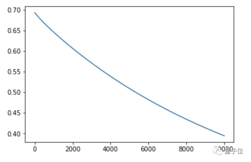
△ 您的成本函数请查收

不过，现在你可能觉得这个算法的代码太多了。为了缩短代码行数，我们用上了scikit学习库。scikit学习库有一个内置的逻辑回归类别，我们可以直接接入使用。

1from sklearn.metrics import accuracy_score
2from sklearn.linear_model import LogisticRegression
3
4clf = LogisticRegression()
5clf.fit(x_train,y_train)
6y_pred = clf.predict(x_test)
7print(accuracy_score(y_test,y_pred))

看，代码已经被缩减到10行以内了。用scikit学习库，我们的模型准确率依然100%。

原文链接：

https://hackernoon.com/introduction-to-machine-learning-algorithms-logistic-regression-cbdd82d81a36

想要了解更多资讯，请扫描下方二维码，关注机器学习研究会

转自：量子位