为此,云朵君教大家自动动手,生成学习时间序列分析和预测过程中,缺少练手数据的问题。当然,大家也可以举一反三,用这样的方法去生成更多适用于其他应用场景的实验数据。
时序数据生成原理
一般而言,数据是由函数生成的,而周期性时间序列数据可以使用由余弦函数来生成。
余弦型函数是实践中广泛应用的一类重要函数,指函数(其中均为常数,且)。这里A称为振幅, 称为圆频率或角频率, 称为初相位或初相角,正弦型函数是周期函数,其周期为。
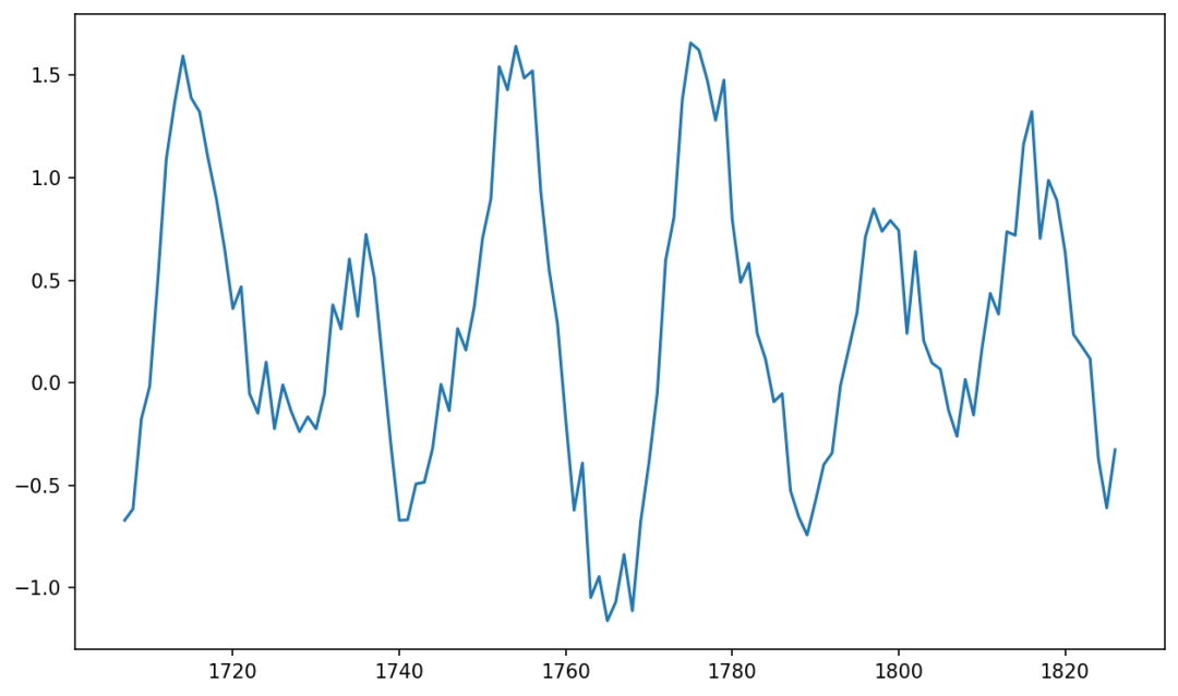
但由于正常的余弦型函数是单调周期性函数,生成的函数图像如下图所示:
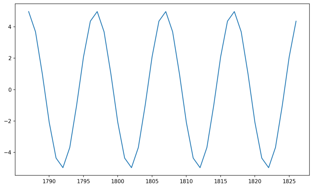
这样的数据太过理想,与现实相差很大。现实中的时序数据具有大量的噪声,因此此时我们只需要加上随机振幅和随机偏移就能生存具有噪声的时间序列数据。
接下来我们一步一步实现具有真实场景的随机时间序列数据。
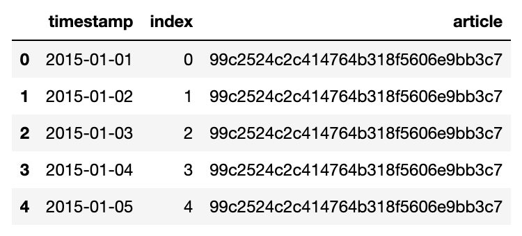
生成时间序列索引
def get_init_df():
    # 生成时间序列索引
    date_rng = pd.date_range(start="2015-01-01", end="2020-01-01", freq="D")
    dataframe = pd.DataFrame(date_rng, columns=["timestamp"])
    dataframe["index"] = range(dataframe.shape[0])
    dataframe["article"] = uuid4().hex
    # UUID 为 32 个字符的十六进制字符串
    return dataframe

get_init_df().head()
设置振幅
生成随机振幅的函数,我们选用
其中:
最后为了增加随机性,每次生成,都有50%的机会正序或倒序排列。
def set_amplitude(dataframe):

    max_step = random.randint(90, 365)
    max_amplitude = random.uniform(0.1, 1)
    offset = random.uniform(-1, 1)

    phase = random.randint(-1000, 1000)

    amplitude = (
        dataframe["index"]
        .apply(lambda x: max_amplitude * (x % max_step + phase) / max_step + offset)
        .values
    )

    # 每次生成,都有50%的机会正序或倒序排列
    if random.random() 0.5:
        amplitude = amplitude[::-1]

    dataframe["amplitude"] = amplitude

    return dataframe
设置偏移
生成随机偏移的函数,我们选用
其中
同样为了增加随机性,每次生成,都有50%的机会正序或倒序排列。
def set_offset(dataframe):
max_step = random.randint(15, 45)
max_offset = random.uniform(-1, 1)
base_offset = random.uniform(-1, 1)
phase = random.randint(-1000, 1000)
offset = (
dataframe["index"]
.apply(
lambda x: max_offset * np.cos(x * 2 * np.pi / max_step + phase)
+ base_offset
)
.values
)
if random.random() 0.5:
offset = offset[::-1]
dataframe[
"offset"] = offset
return dataframe
生成具有噪声的时序数据
生成随机时序数据的函数,我们选用余弦型函数
其中
- 为周期:在 [7, 14, 28, 30] 中随机选择
为了增加随机性,这里有两个细节:
一是设置余弦函数的最大最小值范围,在(0.3, 1)中的随机数。而是在整个函数上加上一系列常数,使得每次生成的数据有一定的差别。该系列常数分布满足是从0到最大振幅之间生成的正态分布。
def generate_time_series(dataframe):
  periods = [7, 14, 28, 30]
    clip_val = random.uniform(0.3, 1)
    period = random.choice(periods)
    phase = random.randint(-1000, 1000)

    dataframe["views"] = dataframe.apply(
        lambda x: np.clip(
            np.cos(x["index"] * 2 * np.pi / period + phase), -clip_val, clip_val
        )
        * x["amplitude"]
        + x["offset"],
        axis=1,
    ) + np.random.normal(
        0, dataframe["amplitude"].abs().max() / 10, size=(dataframe.shape[0],)
    )

    return dataframe
多次生成的数据样式是不同的:
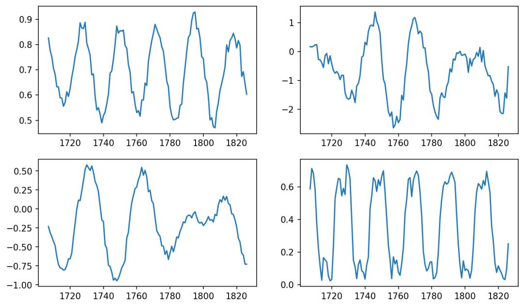
最后我们多次生成,并合并数据:
dataframes = []
for _ in tqdm(range(20)):
  df = generate_df()
  # 简单绘图步骤
  # fig = plt.figure()
  # plt.plot(df[-120:]["index"], df[-120:]["views"])
  # plt.show()

  dataframes.append(df)
  all_data = pd.concat(dataframes, ignore_index=True)
得到如下形状的时间序列数据。

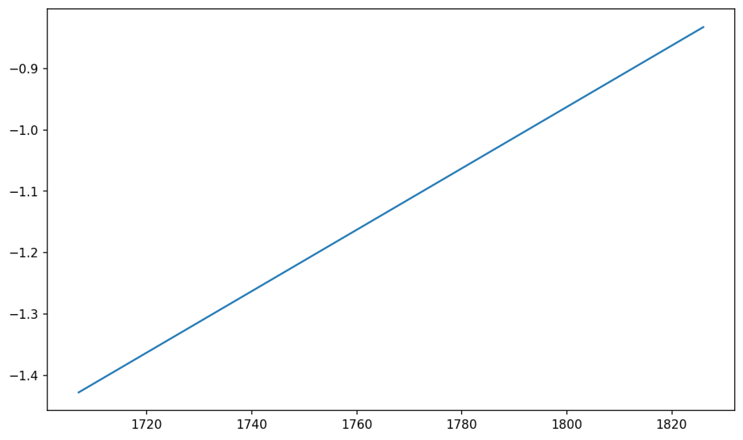
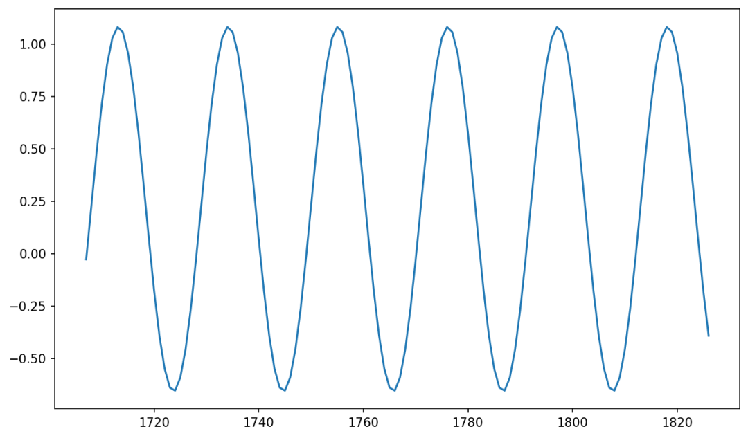
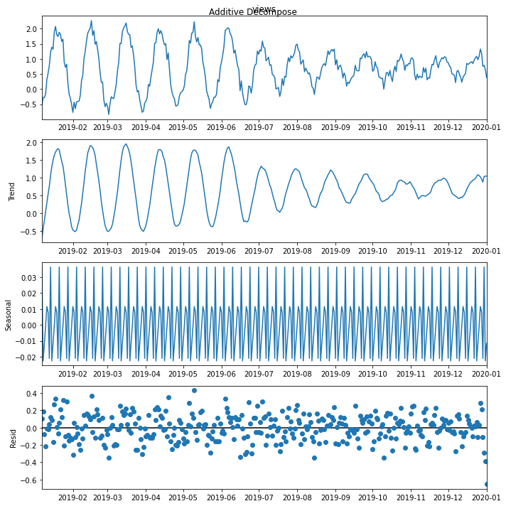
季节性分解
最后,我们使用时间序列季节性分解,看下分解结果。从结果看,基本符合我们日常学习使用。
from statsmodels.tsa.seasonal import seasonal_decompose
df = generate_df()
df = df.set_index(['timestamp'])
result_mul = seasonal_decompose(df['views'],
             model='additive',
             extrapolate_trend='freq')

plt.rcParams.update({'figure.figsize': (10, 10)})
result_mul.plot().suptitle('Additive Decompose')
plt.show()
写在最后
以上就是本次所有内容,本次介绍的所有生成函数中的参数,均可以根据实际需要修改,如最大振幅,最大步长等。

-
- 机器学习交流qq群955171419,加入微信群请
扫码:


