首先我们需要先提前下载好示例数据集:
- drinksbycountry.csv : http://bit.ly/drinksbycountry
- imdbratings.csv : http://bit.ly/imdbratings
- chiporders.csv : http://bit.ly/chiporders
- smallstockers.csv : http://bit.ly/smallstocks
- kaggletrain.csv : http://bit.ly/kaggletrain
- uforeports.csv : http://bit.ly/uforeports
导入案例数据集
import pandas as pd
import numpy as np

drinks = pd.read_csv('http://bit.ly/drinksbycountry')
movies = pd.read_csv('http://bit.ly/imdbratings')
orders = pd.read_csv('http://bit.ly/chiporders', sep='\t')
orders['item_price'] = orders.item_price.str.replace('$', '').astype('float')
stocks = pd.read_csv('http://bit.ly/smallstocks', parse_dates=['Date'])
titanic = pd.read_csv('http://bit.ly/kaggletrain')
ufo = pd.read_csv('http://bit.ly/uforeports', parse_dates=['Time'])
1显示已安装的版本
有时你需要知道正在使用的pandas版本,特别是在阅读pandas文档时。你可以通过输入以下命令来显示pandas版本:
pd.__version__
'0.25.8'
如果你还想知道pandas所依赖的模块的版本,你可以使用show_versions()函数:
pd.show_versions()
INSTALLED VERSIONS
------------------
commit: None
python: 3.7.3.final.0
python-bits: 64
OS: Darwin
OS-release: 18.6.0
machine: x86_64
processor: i386
byteorder: little
LC_ALL: None
LANG: en_US.UTF-8
LOCALE: en_US.UTF-8

pandas: 0.24.2
pytest: None
pip: 19.1.1
setuptools: 41.0.1
Cython: None
numpy: 1.16.4
scipy: None
pyarrow: None
xarray: None
IPython: 7.5.0
sphinx: None
patsy: None
dateutil: 2.8.0
pytz: 2019.1
blosc: None
bottleneck: None
tables: None
numexpr: None
feather: None
matplotlib: 3.1.0
openpyxl: None
xlrd: None
xlwt: None
xlsxwriter: None
lxml.etree: None
bs4: None
html5lib: None
sqlalchemy: None
pymysql: None
psycopg2: None
jinja2: 2.10.1
s3fs: None
fastparquet: None
pandas_gbq: None
pandas_datareader: None
gcsfs: None
你可以查看到Python,pandas, Numpy, matplotlib等的版本信息。
2创建示例DataFrame
假设你需要创建一个示例DataFrame。有很多种实现的途径,我最喜欢的方式是传一个字典给DataFrame constructor,其中字典中的keys为列名,values为列的取值。
df = pd.DataFrame({'col one':[100, 200],
'col two':[300, 400]})
df

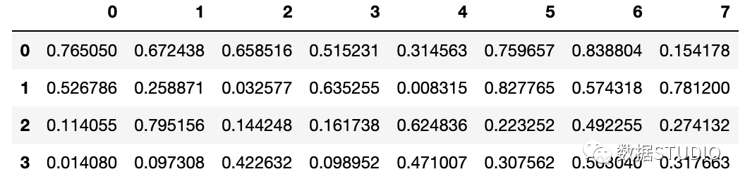
如果你需要更大的DataFrame,上述方法将需要太多的输入。在这种情况下,你可以使用NumPy的 random.rand()函数,定义好该函数的行数和列数,并将其传递给DataFrame构造器:
pd.DataFrame(np.random.rand(4, 8))
这种方式很好,但如果你还想把列名变为非数值型的,你可以强制地将一串字符赋值给columns参数:
pd.DataFrame(np.random.rand(4, 8), columns=list('abcdefgh'))
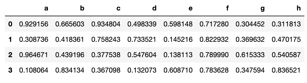
你可以想到,你传递的字符串的长度必须与列数相同。
3更改列名
我们来看一下刚才我们创建的示例DataFrame:
df

我更喜欢在选取pandas列的时候使用点(.),但是这对那么列名中含有空格的列不会生效。让我们来修复这个问题。
更改列名最灵活的方式是使用rename()函数。你可以传递一个字典,其中keys为原列名,values为新列名,还可以指定axis:
df = df.rename({'col one':'col_one',
                'col two':'col_two'},
                axis='columns')
使用这个函数最好的方式是你需要更改任意数量的列名,不管是一列或者全部的列。
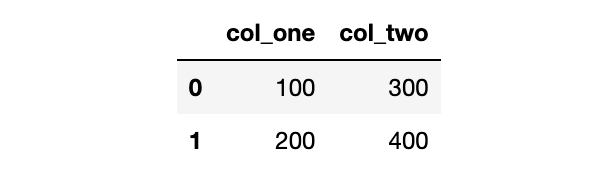
如果你需要一次性重新命令所有的列名,更简单的方式就是重写DataFrame的columns属性:
df.columns = ['col_one', 'col_two']
如果你需要做的仅仅是将空格换成下划线,那么更好的办法是用str.replace()方法,这是因为你都不需要输入所有的列名:
df.columns = df.columns.str.replace(' ', '_')
上述三个函数的结果都一样,可以更改列名使得列名中不含有空格:
df
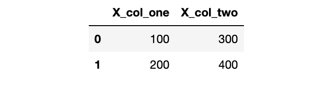
最后,如果你需要在列名中添加前缀或者后缀,你可以使用
add_prefix()函数:
df.add_prefix('X_')
或者使用add_suffix()函数:
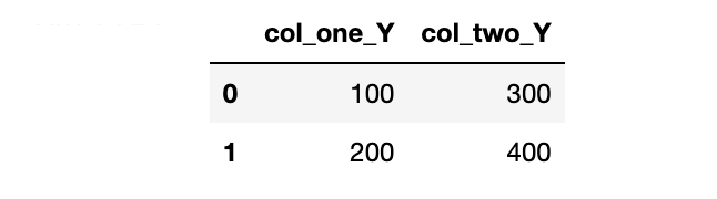
df.add_suffix('_Y')
4. 行序反转
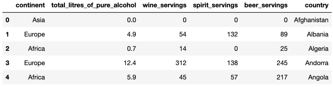
我们来看一下drinks这个DataFame:
drinks.head()
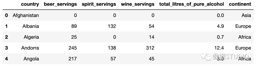
该数据集描述了每个国家的平均酒消费量。如果你想要将行序反转呢?
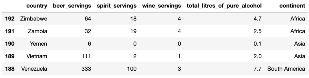
最直接的办法是使用loc函数并传递::-1,跟Python中列表反转时使用的切片符号一致:
drinks.loc[::-1].head()
如果你还想重置索引使得它从0开始呢?
你可以使用reset_index()函数,告诉他去掉完全抛弃之前的索引:
drinks.loc[::-1].reset_index(drop=True).head()
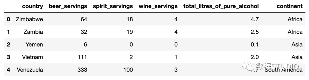
你可以看到,行序已经反转,索引也被重置为默认的整数序号。
5. 列序反转
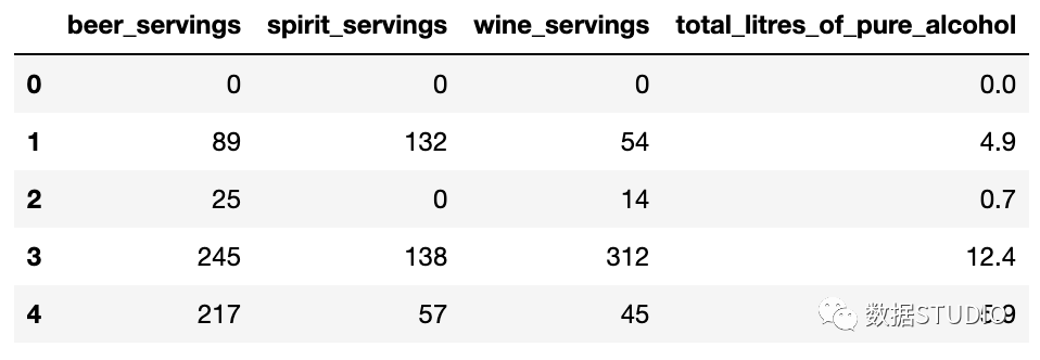
跟之前的技巧一样,你也可以使用loc函数将列从左至右反转
drinks.loc[:, ::-1].head()
逗号之前的冒号表示选择所有行,逗号之后的::-1表示反转所有的列,这就是为什么country这一列现在在最右边。
6. 通过数据类型选择列
这里有drinks这个DataFrame的数据类型:
drinks.dtypes
country                          object
beer_servings                     int64
spirit_servings                   int64
wine_servings                     int64
total_litres_of_pure_alcohol    float64
continent                        object
dtype: object
假设你仅仅需要选取数值型的列,那么你可以使用select_dtypes()函数:
drinks.select_dtypes(include='number').head()
这包含了int和float型的列。
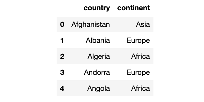
你也可以使用这个函数来选取数据类型为object的列:
drinks.select_dtypes(include='object').head()
你还可以选取多种数据类型,只需要传递一个列表即可:
drinks.select_dtypes(include=['number', 'object', 'category', 'datetime']).head()
你还可以用来排除特定的数据类型:
drinks.select_dtypes(exclude='number').head()

7. 将字符型转换为数值型
我们来创建另一个示例DataFrame:
df = pd.DataFrame({'col_one':['1.1', '2.2', '3.3'],
                   'col_two':['4.4', '5.5', '6.6'],
                   'col_three':['7.7', '8.8', '-']})
df
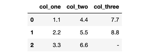
这些数字实际上储存为字符型,导致其数据类型为object:
df.dtypes
col_one      object
col_two      object
col_three    object
dtype: object
为了对这些列进行数学运算,我们需要将数据类型转换成数值型。你可以对前两列使用astype()函数:
df.astype({'col_one':'float', 'col_two':'float'}).dtypes
col_one float64
col_two float64
col_three object
dtype: object
但是,如果你对第三列也使用这个函数,将会引起错误,这是因为这一列包含了破折号(用来表示0)但是pandas并不知道如何处理它。
你可以对第三列使用to_numeric()函数,告诉其将任何无效数据转换为NaN:
pd.to_numeric(df.col_three, errors='coerce')
0    7.7
1    8.8
2    NaN
Name: col_three, dtype: float64
如果你知道NaN值代表0,那么你可以fillna()函数将他们替换成0:
pd.to_numeric(df.col_three, errors='coerce').fillna(0)
0    7.7
1    8.8
2    0.0
Name: col_three, dtype: float64
最后,你可以通过apply()函数一次性对整个DataFrame使用这个函数:
df = df.apply(pd.to_numeric, errors='coerce').fillna(0)
df
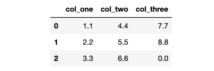
仅需一行代码就完成了我们的目标,因为现在所有的数据类型都转换成float:
df.dtypes
col_one      float64
col_two      float64
col_three    float64
dtype: object
8. 减小DataFrame空间大小
pandas DataFrame被设计成可以适应内存,所以有些时候你可以减小DataFrame的空间大小,让它在你的系统上更好地运行起来。
这是drinks这个DataFrame所占用的空间大小:
drinks.info(memory_usage='deep')
RangeIndex: 193 entries, 0 to 192
Data columns (total 6 columns):
country                         193 non-null object
beer_servings                   193 non-null int64
spirit_servings                 193 non-null int64
wine_servings                   193 non-null int64
total_litres_of_pure_alcohol    193 non-null float64
continent                       193 non-null object
dtypes: float64(1), int64(3), object(2)
memory usage: 30.4 KB
可以看到它使用了304.KB。
如果你对你的DataFrame有操作方面的问题,或者你不能将它读进内存,那么在读取文件的过程中有两个步骤可以使用来减小DataFrame的空间大小。
第一个步骤是只读取那些你实际上需要用到的列,可以调用usecols参数:
cols = ['beer_servings', 'continent']
small_drinks = pd.read_csv('http://bit.ly/drinksbycountry', usecols=cols)
small_drinks.info(memory_usage='deep')
RangeIndex: 193 entries, 0 to 192
Data columns (total 2 columns):
beer_servings    193 non-null int64
continent        193 non-null object
dtypes: int64(1), object(1)
memory usage: 13.6 KB
通过仅读取用到的两列,我们将DataFrame的空间大小缩小至13.6KB。
第二步是将所有实际上为类别变量的object列转换成类别变量,可以调用dtypes参数:
dtypes = {'continent':'category'}
smaller_drinks = pd.read_csv('http://bit.ly/drinksbycountry', usecols=cols, dtype=dtypes)
smaller_drinks.info(memory_usage='deep')
RangeIndex: 193 entries, 0 to 192
Data columns (total 2 columns):
beer_servings    193 non-null int64
continent        193 non-null category
dtypes: category(1), int64(1)
memory usage: 2.3 KB
通过将continent列读取为category数据类型,我们进一步地把DataFrame的空间大小缩小至2.3KB。
值得注意的是,如果跟行数相比,category数据类型的列数相对较小,那么catefory数据类型可以减小内存占用。
9. 按行从多个文件中构建DataFrame
假设你的数据集分化为多个文件,但是你需要将这些数据集读到一个DataFrame中。
举例来说,我有一些关于股票的小数聚集,每个数据集为单天的CSV文件。
pd.read_csv('data/stocks1.csv')
pd.read_csv('data/stocks2.csv')
pd.read_csv('data/stocks3.csv')
你可以将每个CSV文件读取成DataFrame,将它们结合起来,然后再删除原来的DataFrame,但是这样会多占用内存且需要许多代码。
更好的方式为使用内置的glob模块。你可以给glob()函数传递某种模式,包括未知字符,这样它会返回符合该某事的文件列表。在这种方式下,glob会查找所有以stocks开头的CSV文件:
from glob import glob

stock_files = sorted(glob('data/stocks*.csv'))
stock_files
['data/stocks1.csv', 'data/stocks2.csv', 'data/stocks3.csv']
glob会返回任意排序的文件名,这就是我们为什么要用Python内置的sorted()函数来对列表进行排序。
我们以生成器表达式用read_csv()函数来读取每个文件,并将结果传递给concat()函数,这会将单个的DataFrame按行来组合:
pd.concat((pd.read_csv(file) for file in stock_files))
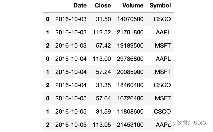
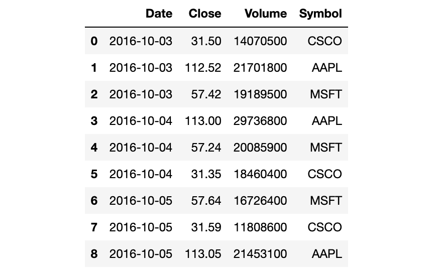
不幸的是,索引值存在重复。为了避免这种情况,我们需要告诉concat()函数来忽略索引,使用默认的整数索引:
pd.concat((pd.read_csv(file) for file in stock_files), ignore_index=True)
10. 按列从多个文件中构建DataFrame
上一个技巧对于数据集中每个文件包含行记录很有用。但是如果数据集中的每个文件包含的列信息呢?
这里有一个例子,dinks数据集被划分成两个CSV文件,每个文件包含三列:
pd.read_csv('data/drinks1.csv').head()
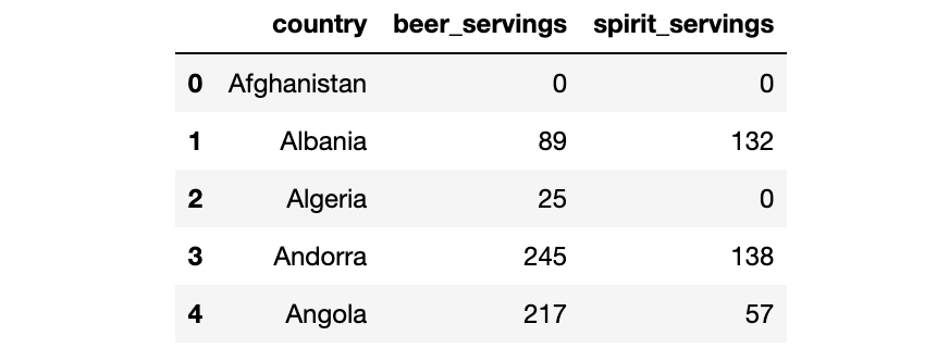
pd.read_csv('data/drinks2.csv').head()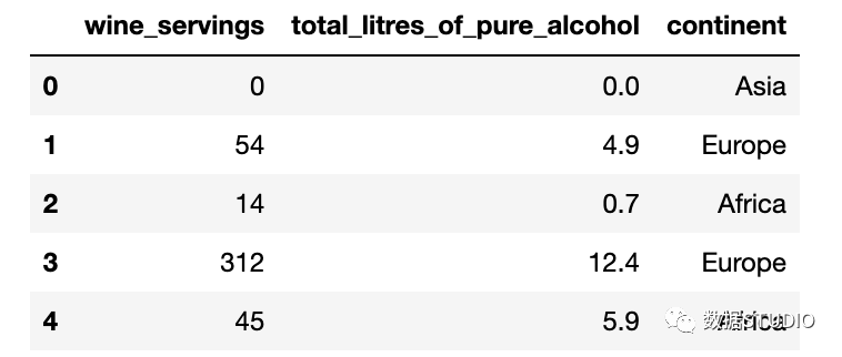
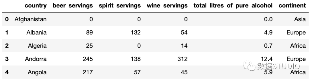
同上一个技巧一样,我们以使用glob()函数开始。这一次,我们需要告诉concat()函数按列来组合:
drink_files = sorted(glob('data/drinks*.csv'))
pd.concat((pd.read_csv(file) for file in drink_files), axis='columns').head()
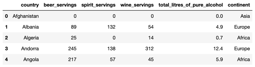
现在我们的DataFrame已经有六列了。
11. 从剪贴板中创建DataFrame
假设你将一些数据储存在Excel或者Google Sheet中,你又想要尽快地将他们读取至DataFrame中。
你需要选择这些数据并复制至剪贴板。然后,你可以使用read_clipboard()函数将他们读取至DataFrame中:
df = pd.read_clipboard()
df
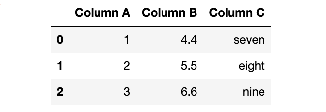
和read_csv()类似,read_clipboard()会自动检测每一列的正确的数据类型:
df.dtypes
Column A      int64
Column B    float64
Column C     object
dtype: object
我们再复制另外一个数据至剪贴板:
df = pd.read_clipboard()
df
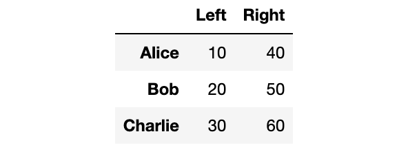
神奇的是,pandas已经将第一列作为索引了:
df.index
Index(['Alice', 'Bob', 'Charlie'], dtype='object')
需要注意的是,如果你想要你的工作在未来可复制,那么read_clipboard()并不值得推荐。
12. 将DataFrame划分为两个随机的子集
假设你想要将一个DataFrame划分为两部分,随机地将75%的行给一个DataFrame,剩下的25%的行给另一个DataFrame。
举例来说,我们的movie ratings这个DataFrame有979行:
len(movies)
979
12. 将DataFrame划分为两个随机的子集
假设你想要将一个DataFrame划分为两部分,随机地将75%的行给一个DataFrame,剩下的25%的行给另一个DataFrame。
举例来说,我们的movie ratings这个DataFrame有979行:
movies_1 = movies.sample(frac=0.75, random_state=1234)
接着我们使用drop()函数来舍弃“moive_1”中出现过的行,将剩下的行赋值给"movies_2"DataFrame:
movies_2 = movies.drop(movies_1.index)
你可以发现总的行数是正确的:
len(movies_1) + len(movies_2)
979
你还可以检查每部电影的索引,或者"moives_1":
movies_1.index.sort_values()
Int64Index([  0,   2,   5,   6,   7,   8,   9,  11,  13,  16,
            ...
            966, 967, 969, 971, 972, 974, 975, 976, 977, 978],
           dtype='int64', length=734)
或者"moives_2":
movies_2.index.sort_values()
Int64Index([  1,   3,   4,  10,  12,  14,  15,  18,  26,  30,
            ...
            931, 934, 937, 941, 950, 954, 960, 968, 970, 973],
           dtype='int64', length=245)
需要注意的是,这个方法在索引值不唯一的情况下不起作用。
读者注:该方法在机器学习或者深度学习中很有用,因为在模型训练前,我们往往需要将全部数据集按某个比例划分成训练集和测试集。该方法既简单又高效,值得学习和尝试。
13. 通过多种类型对DataFrame进行过滤
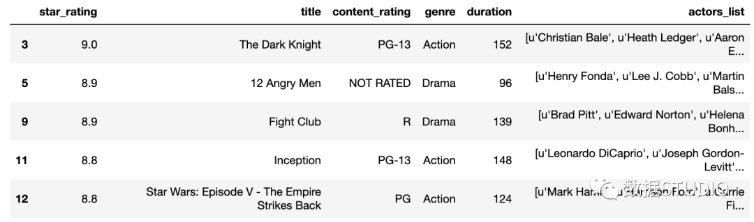
我们先看一眼movies这个DataFrame:
movies.head()
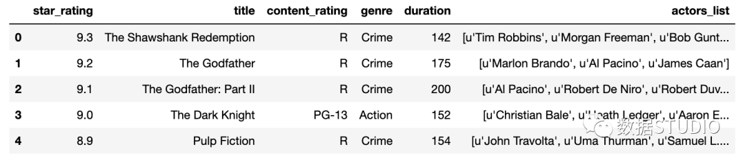
其中有一列是genre(类型):
movies.genre.unique()
array(['Crime', 'Action', 'Drama', 'Western', 'Adventure', 'Biography',
       'Comedy', 'Animation', 'Mystery', 'Horror', 'Film-Noir', 'Sci-Fi',
       'History', 'Thriller', 'Family', 'Fantasy'], dtype=object)
比如我们想要对该DataFrame进行过滤,我们只想显示genre为Action或者Drama或者Western的电影,我们可以使用多个条件,以"or"符号分隔
movies[(movies.genre == 'Action') |
       (movies.genre == 'Drama') |
       (movies.genre == 'Western')].head()
但是,你实际上可以使用isin()函数将代码写得更加清晰,将genres列表传递给该函数:
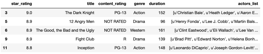
movies[movies.genre.isin(['Action', 'Drama', 'Western'])].head()

如果你想要进行相反的过滤,也就是你将吧刚才的三种类型的电影排除掉,那么你可以在过滤条件前加上破浪号:
movies[~movies.genre.isin(['Action', 'Drama', 'Western'])].head()
这种方法能够起作用是因为在Python中,波浪号表示“not”操作。
14. 从DataFrame中筛选出数量最多的类别
假设你想要对movies这个DataFrame通过genre进行过滤,但是只需要前3个数量最多的genre。
我们对genre使用value_counts()函数,并将它保存成counts(type为Series):
counts = movies.genre.value_counts()
counts
Drama        278
Comedy       156
Action       136
Crime        124
Biography     77
Adventure     75
Animation     62
Horror        29
Mystery       16
Western        9
Sci-Fi         5
Thriller       5
Film-Noir      3
Family         2
Fantasy        1
History        1
Name: genre, dtype: int64
该Series的nlargest()函数能够轻松地计算出Series中前3个最大值:
counts.nlargest(3)
Drama     278
Comedy    156
Action    136
Name: genre, dtype: int64
事实上我们在该Series中需要的是索引:
counts.nlargest(3).index
Index(['Drama', 'Comedy', 'Action'], dtype='object')
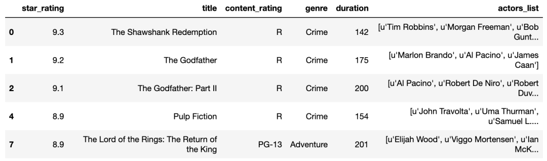
最后,我们将该索引传递给isin()函数,该函数会把它当成genre列表:
movies[movies.genre.isin(counts.nlargest(3).index)].head()
样,在DataFrame中只剩下Drame, Comdey, Action这三种类型的电影了。
15. 处理缺失值
我们来看一看UFO sightings这个DataFrame:
ufo.head()
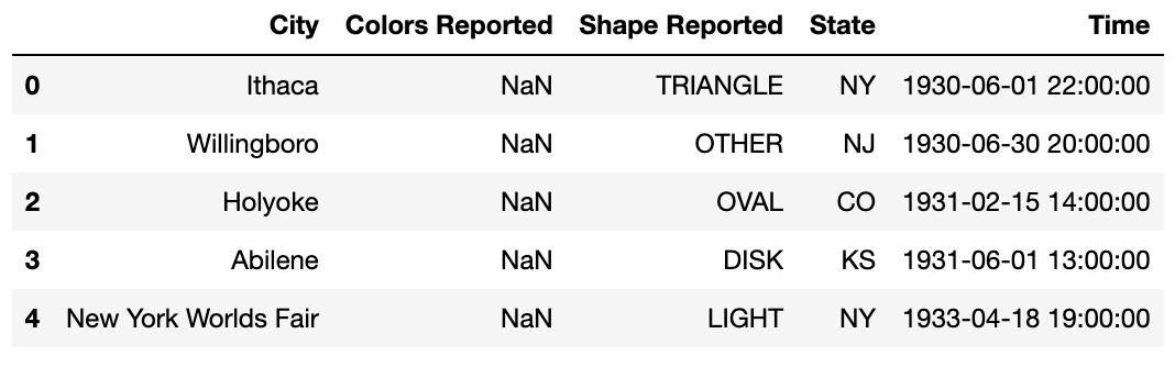
你将会注意到有些值是缺失的。 为了找出每一列中有多少值是缺失的,你可以使用isna()函数,然后再使用sum():
ufo.isna().sum()
City                  25
Colors Reported    15359
Shape Reported      2644
State                  0
Time                   0
dtype: int64
isna()
会产生一个由True和False组成的DataFrame,sum()会将所有的True值转换为1,False转换为0并把它们加起来。
类似地,你可以通过mean()和isna()函数找出每一列中缺失值的百分比。
ufo.isna().mean()
City               0.001371
Colors Reported    0.842004
Shape Reported     0.144948
State              0.000000
Time               0.000000
dtype: float64
如果你想要舍弃那些包含了缺失值的列,你可以使用dropna()函数:
ufo.dropna(axis='columns').head()
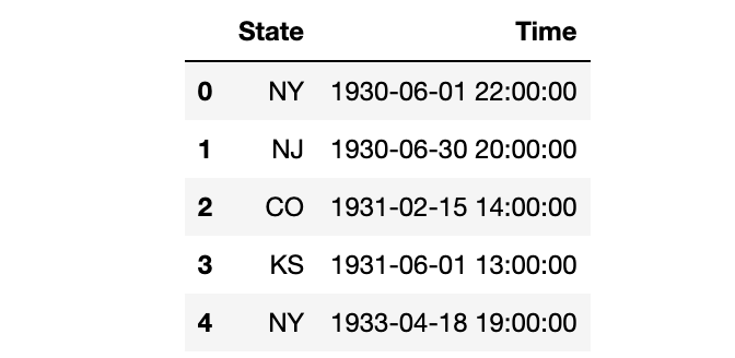
或者你想要舍弃那么缺失值占比超过10%的列,你可以给dropna()设置一个阈值:
ufo.dropna(thresh=len(ufo)*0.9, axis='columns').head()
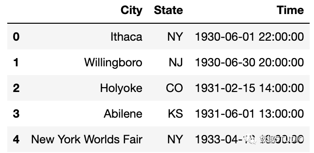
len(ufo)返回总行数,我们将它乘以0.9,以告诉pandas保留那些至少90%的值不是缺失值的列。
16. 将一个字符串划分成多个列
我们先创建另一个新的示例DataFrame:
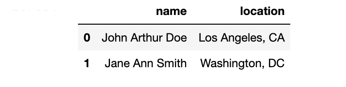
df = pd.DataFrame({'name':['John Arthur Doe', 'Jane Ann Smith'],
                   'location':['Los Angeles, CA', 'Washington, DC']})
df
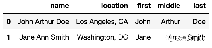
如果我们需要将“name”这一列划分为三个独立的列,用来表示first, middle, last name呢?我们将会使用str.split()函数,告诉它以空格进行分隔,并将结果扩展成一个DataFrame:
df.name.str.split(' ', expand=True)

这三列实际上可以通过一行代码保存至原来的DataFrame:
df[['first', 'middle', 'last']] = df.name.str.split(' ', expand=True)
df
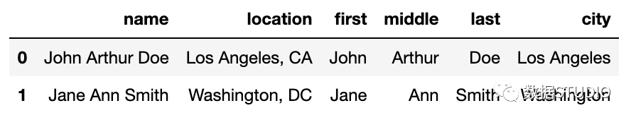
如果我们想要划分一个字符串,但是仅保留其中一个结果列呢?比如说,让我们以", "来划分location这一列:
df.location.str.split(', ', expand=True)

如果我们只想保留第0列作为city name,我们仅需要选择那一列并保存至DataFrame:
df['city'] = df.location.str.split(', ', expand=True)[0]
df
17. 将一个由列表组成的Series扩展成DataFrame
我们创建一个新的示例DataFrame:
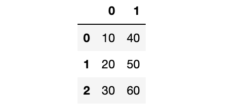
df = pd.DataFrame({'col_one':['a', 'b', 'c'], 'col_two':[[10, 40], [20, 50], [30, 60]]})
df
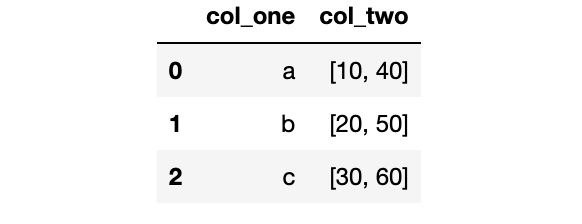
这里有两列,第二列包含了Python中的由整数元素组成的列表。
如果我们想要将第二列扩展成DataFrame,我们可以对那一列使用apply()函数并传递给Series constructor:
df_new = df.col_two.apply(pd.Series)
df_new
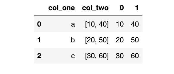
通过使用concat()函数,我们可以将原来的DataFrame和新的DataFrame组合起来:
pd.concat([df, df_new], axis='columns')
18. 对多个函数进行聚合
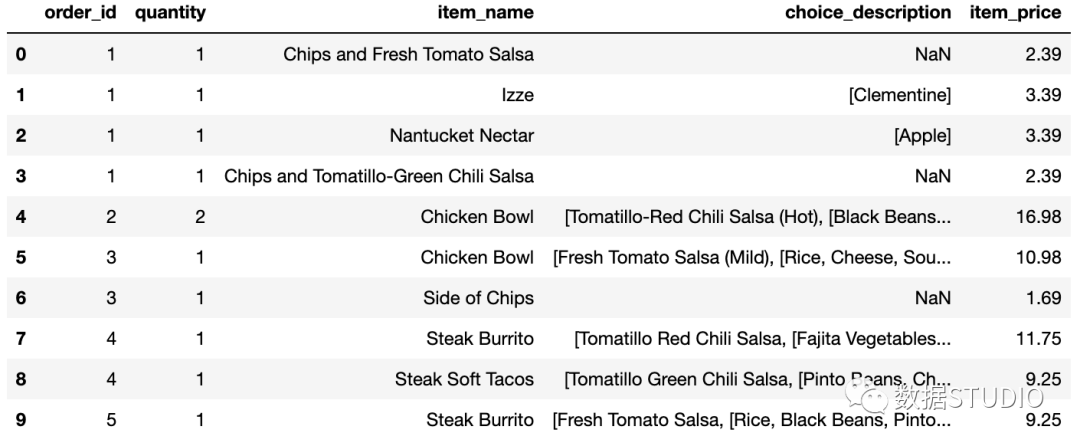
我们来看一眼从Chipotle restaurant chain得到的orders这个DataFrame:
orders.head(10)
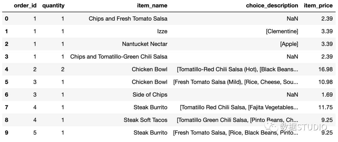
每个订单(order)都有订单号(order_id),包含一行或者多行。为了找出每个订单的总价格,你可以将那个订单号的价格(item_price)加起来。比如,这里是订单号为1的总价格:
orders[orders.order_id == 1].item_price.sum()
11.56
如果你想要计算每个订单的总价格,你可以对order_id使用groupby(),再对每个group的item_price进行求和。
orders.groupby('order_id').item_price.sum().head()
order_id
1    11.56
2    16.98
3    12.67
4    21.00
5    13.70
Name: item_price, dtype: float64
但是,事实上你不可能在聚合时仅使用一个函数,比如sum()。为了对多个函数进行聚合,你可以使用agg()函数,传给它一个函数列表,比如sum()和count():
orders.groupby('order_id').item_price.agg(['sum', 'count']).head()
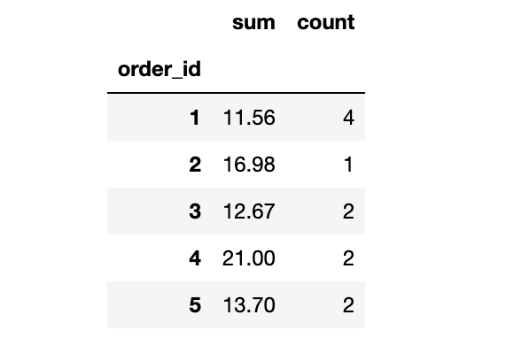
这将告诉我们没定订单的总价格和数量。
19. 将聚合结果与DataFrame进行组合
我们再看一眼orders这个DataFrame:
orders.head(10)
如果我们想要增加新的一列,用于展示每个订单的总价格呢?回忆一下,我们通过使用sum()函数得到了总价格:
orders.groupby('order_id').item_price.sum().head()
order_id
1    11.56
2    16.98
3    12.67
4    21.00
5    13.70
Name: item_price, dtype: float64
sum()是一个聚合函数,这表明它返回输入数据的精简版本(reduced version )。
换句话说,sum()函数的输出:
len(orders.groupby('order_id').item_price.sum())
1834
比这个函数的输入要小:
len(orders.item_price)
4622
解决的办法是使用transform()函数,它会执行相同的操作但是返回与输入数据相同的形状:
total_price = orders.groupby('order_id').item_price.transform('sum')
len(total_price)
4622
我们将这个结果存储至DataFrame中新的一列:
orders['total_price'] = total_price
orders.head(10)
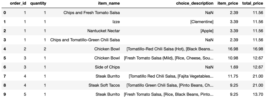
你可以看到,每个订单的总价格在每一行中显示出来了。
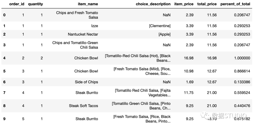
这样我们就能方便地甲酸每个订单的价格占该订单的总价格的百分比:
orders['percent_of_total'] = orders.item_price / orders.total_price
orders.head(10)
20. 选取行和列的切片
我们看一眼另一个数据集:
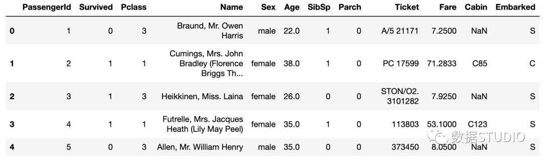
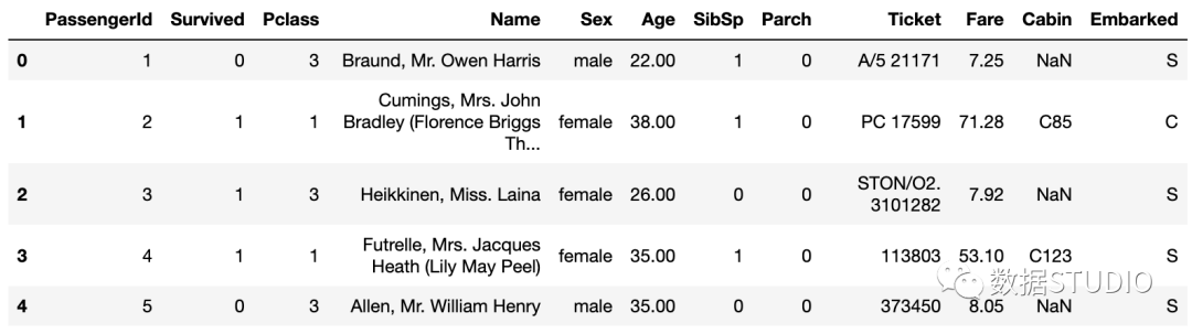
titanic.head()
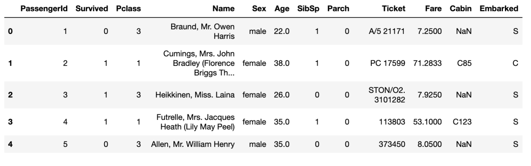
这就是著名的Titanic数据集,它保存了Titanic上乘客的信息以及他们是否存活。
如果你想要对这个数据集做一个数值方面的总结,你可以使用describe()函数:
titanic.describe()
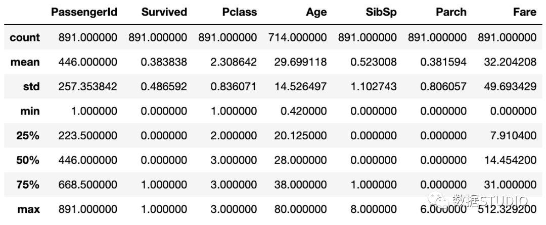
但是,这个DataFrame结果可能比你想要的信息显示得更多。
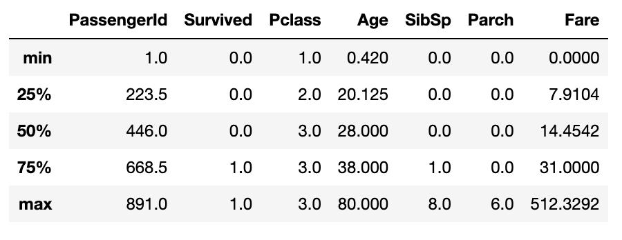
如果你想对这个结果进行过滤,只想显示“五数概括法”(five-number summary)的信息,你可以使用loc函数并传递"min"到"max"的切片:
titanic.describe().loc['min':'max']
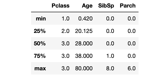
如果你不是对所有列都感兴趣,你也可以传递列名的切片:
titanic.describe().loc['min':'max', 'Pclass':'Parch']
21. 对MultiIndexed Series进行重塑
Titanic数据集的Survived列由1和0组成,因此你可以对这一列计算总的存活率:
titanic.Survived.mean()
0.3838383838383838
如果你想对某个类别,比如“Sex”,计算存活率,你可以使用groupby():
titanic.groupby('Sex').Survived.mean()
Sex
female    0.742038
male      0.188908
Name: Survived, dtype: float64
如果你想一次性对两个类别变量计算存活率,你可以对这些类别变量使用groupby():
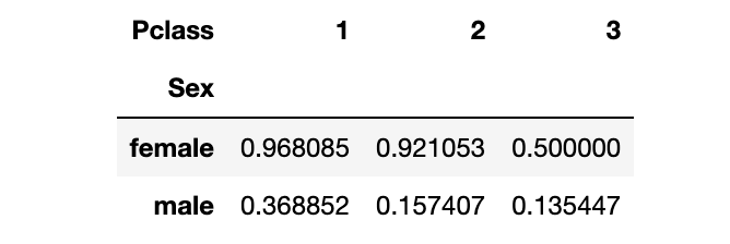
titanic.groupby(['Sex', 'Pclass']).Survived.mean()
Sex     Pclass
female  1         0.968085
        2         0.921053
        3         0.500000
male    1         0.368852
        2         0.157407
        3         0.135447
Name: Survived, dtype: float64
该结果展示了由Sex和Passenger Class联合起来的存活率。它存储为一个MultiIndexed Series,也就是说它对实际数据有多个索引层级。
这使得该数据难以读取和交互,因此更为方便的是通过unstack()函数将MultiIndexed Series重塑成一个DataFrame:
titanic.groupby(['Sex', 'Pclass']).Survived.mean().unstack()
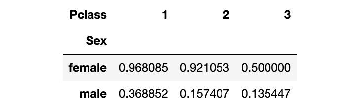
该DataFrame包含了与MultiIndexed Series一样的数据,不同的是,现在你可以用熟悉的DataFrame的函数对它进行操作。
22. 创建数据透视表(pivot table)
如果你经常使用上述的方法创建DataFrames,你也许会发现用pivot_table()函数更为便捷:
titanic.pivot_table(index='Sex', columns='Pclass', values='Survived', aggfunc='mean')
想要使用数据透视表,你需要指定索引(index), 列名(columns), 值(values)和聚合函数(aggregation function)。
数据透视表的另一个好处是,你可以通过设置margins=True轻松地将行和列都加起来:
titanic.pivot_table(index='Sex', columns='Pclass', values='Survived', aggfunc='mean',
                    margins=True)
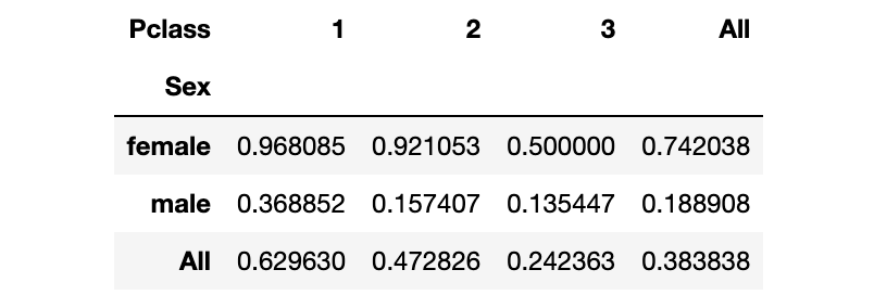
T这个结果既显示了总的存活率,也显示了Sex和Passenger Class的存活率。
最后,你可以创建交叉表(cross-tabulation),只需要将聚合函数由"mean"改为"count":
titanic.pivot_table(index='Sex', columns='Pclass', values='Survived', aggfunc='count',
                    margins=True)
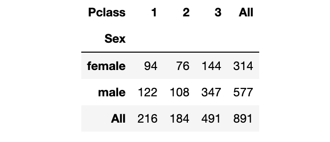
这个结果展示了每一对类别变量组合后的记录总数。
23. 将连续数据转变成类别数据
我们来看一下Titanic数据集中的Age那一列:
titanic.Age.head(10)
0    22.0
1    38.0
2    26.0
3    35.0
4    35.0
5     NaN
6    54.0
7     2.0
8    27.0
9    14.0
Name: Age, dtype: float64
它现在是连续性数据,但是如果我们想要将它转变成类别数据呢?
一个解决办法是对年龄范围打标签,比如"adult", "young adult", "child"。实现该功能的最好方式是使用cut()函数:
pd.cut(titanic.Age, bins=[0, 18, 25, 99], labels=['child', 'young adult', 'adult']).head(10)
0    young adult
1          adult
2          adult
3          adult
4          adult
5            NaN
6          adult
7          child
8          adult
9          child
Name: Age, dtype: category
Categories (3, object): [child < young adult < adult]
这会对每个值打上标签。0到18岁的打上标签"child",18-25岁的打上标签"young adult",25到99岁的打上标签“adult”。
注意到,该数据类型为类别变量,该类别变量自动排好序了(有序的类别变量)。
24. 更改显示选项
我们再来看一眼Titanic 数据集:
titanic.head()
注意到,Age列保留到小数点后1位,Fare列保留到小数点后4位。如果你想要标准化,将显示结果保留到小数点后2位呢?
你可以使用set_option()函数:
pd.set_option('display.float_format', '{:.2f}'.format)

titanic.head()
set_option()函数中第一个参数为选项的名称,第二个参数为Python格式化字符。可以看到,Age列和Fare列现在已经保留小数点后两位。注意,这并没有修改基础的数据类型,而只是修改了数据的显示结果。
你也可以重置任何一个选项为其默认值:
pd.reset_option('display.float_format')
对于其它的选项也是类似的使用方法。
25. Style a DataFrame
上一个技巧在你想要修改整个jupyter notebook中的显示会很有用。但是,一个更灵活和有用的方法是定义特定DataFrame中的格式化(style)。
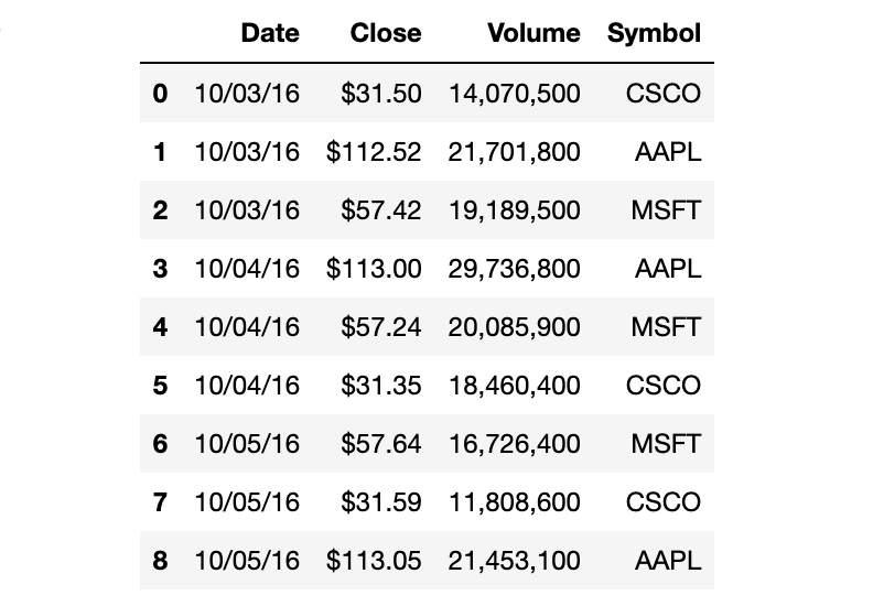
我们回到stocks这个DataFrame:
stocks

我们可以创建一个格式化字符串的字典,用于对每一列进行格式化。然后将其传递给DataFrame的style.format()函数:
format_dict = {'Date':'{:%m/%d/%y}', 'Close'
:'${:.2f}', 'Volume':'{:,}'}
stocks.style.format(format_dict)
注意到,Date列是month-day-year的格式,Close列包含一个$符号,Volume列包含逗号。
我们可以通过链式调用函数来应用更多的格式化:
(stocks.style.format(format_dict)
 .hide_index()
 .highlight_min('Close', color='red')
 .highlight_max('Close', color='lightgreen')
)
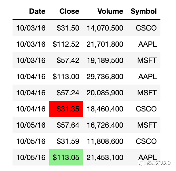
我们现在隐藏了索引,将Close列中的最小值高亮成红色,将Close列中的最大值高亮成浅绿色。
这里有另一个DataFrame格式化的例子:
(stocks.style.format(format_dict)
 .hide_index()
 .background_gradient(subset='Volume', cmap='Blues')
)
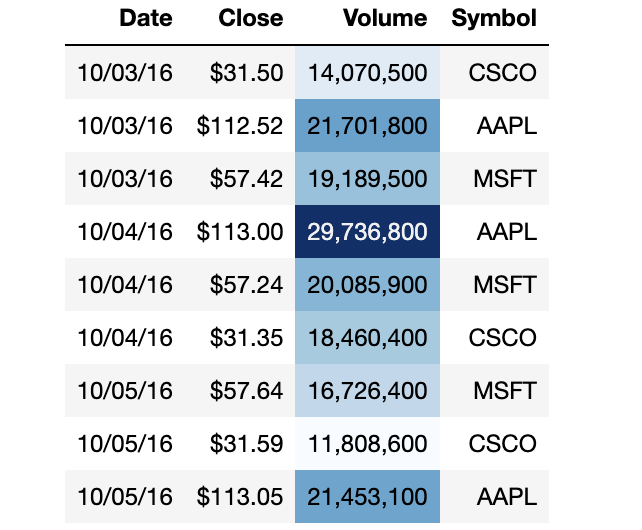
Volume列现在有一个渐变的背景色,你可以轻松地识别出大的和小的数值。
最后一个例子:
(stocks.style.format(format_dict)
 .hide_index()
 .bar('Volume', color='lightblue', align='zero')
 .set_caption('Stock Prices from October 2016')
)
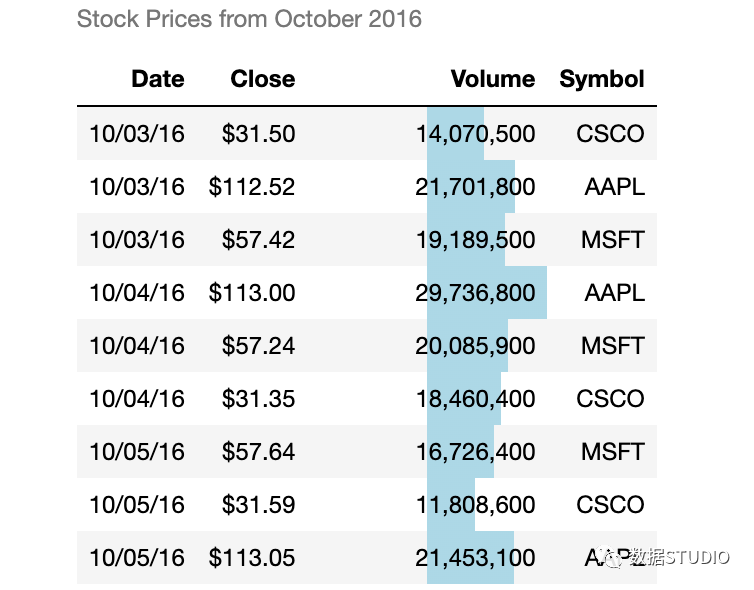
现在,Volumn列上有一个条形图,DataFrame上有一个标题。请注意,还有许多其他的选项你可以用来格式化DataFrame。
额外技巧:Profile a DataFrame
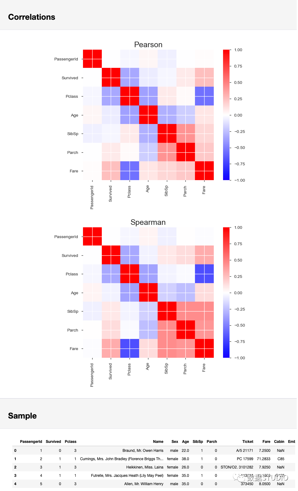
假设你拿到一个新的数据集,你不想要花费太多力气,只是想快速地探索下。那么你可以使用pandas-profiling这个模块。在你的系统上安装好该模块,然后使用ProfileReport()函数,传递的参数为任何一个DataFrame。它会返回一个互动的HTML报告:
- 第一部分为该数据集的总览,以及该数据集可能出现的问题列表;
- 第二部分为每一列的总结。你可以点击"toggle details"获取更多信息;
使用示例如下(只显示第一部分的报告):
import pandas_profiling
pandas_profiling.ProfileReport(titanic)
- 机器学习交流qq群955171419,加入微信群请扫码


