去年一月份,根据某项目的要求,我们需要从预报的WRFOUT文件中提取500mb等压线、风羽集合、等压线集合以及台风路径,并以json文件格式呈现。这种json文件可以直接在网页端显示,或者在我们自行创建的系统中展示。它具有较高的地理匹配度,与以往使用Python绘制图片的方法有明显不同。我将提供处理500mb等压线等内容的代码注解,所有代码都将通过百度网盘分享。
首先是导入各种python库:
import xarray as xrimport numpy as npimport mathimport netCDF4 as ncfrom netCDF4 import Dataset,num2date,date2numfrom wrf import getvar,ll_to_xy,interplevel,vinterp,get_cartopy,latlon_coords,cartopy_xlim,cartopy_ylimfrom math import atan2,piimport pandas as pdimport datetimeimport wrf import geopandas as gpdimport salemfrom salem.utils import get_demo_filefrom matplotlib import colorsimport matplotlib.pyplot as pltimport matplotlib as mplfrom datetime import datetime,timedeltafrom cartopy.io.shapereader import Readerimport cartopy.crs as crsimport matplotlib.ticker as mtickerfrom salem.utils import get_demo_filefrom scipy.interpolate import griddatafrom salem import cache_dir, sample_data_dirimport json
其次通过读取WRFOUT数据提取500mb等高线、风羽集合、等压线集合的数据:
Ht_500mb=[]Wspd10=[]Wdir10=[]Slp=[]timerange=pd.date_range(start='2019-08-05 18:00:00',end='2019-08-11 12:00:00',freq='H')for t in range(0,len(timerange),6): print(str(timerange[t])) t1=str(timerange[t]).replace(' ','_').replace(':','_') ncfile = Dataset("./wrfout_d02_2019-08-05_18:00:00") lat=getvar(ncfile, "XLAT",timeidx=0).data lon=getvar(ncfile, "XLONG",timeidx=0).data time=getvar(ncfile,"times",timeidx=t).data z = getvar(ncfile, "z",timeidx=t) p = getvar(ncfile, "pressure",timeidx=t) # Compute the 500 MB Geopotential Height ht_500mb = (interplevel(z, p, 500.)/10).data slp=getvar(ncfile,"slp",timeidx=t).data wspd10=getvar(ncfile,"wspd10",timeidx=t).data wdir10=getvar(ncfile,"wdir10",timeidx=t).data llat1=np.arange(1.51,40.34,0.03)
llon1=np.arange(108.00,130.93,0.03) llon,llat=np.meshgrid(llon1,llat1)
llat2=np.arange(1.51,40.34,1) llon2=np.arange(108.00,130.93,1)
llon_wind,llat_wind=np.meshgrid(llon2,llat2) #插值数据到指定的经纬度 ht_500mb_grid=griddata((lat.ravel(),lon.ravel()),ht_500mb.ravel(),(llat,llon), method='linear') wspd10_grid=griddata((lat.ravel(),lon.ravel()),wspd10.ravel(),(llat_wind,llon_wind), method='linear') wdir10_grid=griddata((lat.ravel(),lon.ravel()),wdir10.ravel(),(llat_wind,llon_wind), method='linear') slp_grid=griddata((lat.ravel(),lon.ravel()),slp.ravel(),(llat,llon), method='linear') Ht_500mb.append(ht_500mb_grid[np.newaxis,:]) Wspd10.append(wspd10_grid[np.newaxis,:]) Wdir10.append(wdir10_grid[np.newaxis,:]) Slp.append(slp_grid[np.newaxis,:])Ht_500mb=np.concatenate(Ht_500mb, axis=0)Wspd10=np.concatenate(Wspd10, axis=0)Wdir10=np.concatenate(Wdir10, axis=0)Slp=np.concatenate(Slp, axis=0)
timerange=pd.date_range(start='2019-08-05 18:00:00',end='2019-08-11 12:00:00',freq='6H')ht500mb=xr.Dataset()ht500mb['time']=(['time'],timerange)ht500mb['latitude']=(['latitude'],llat1)ht500mb['longitude']=(['longitude'],llon1)ht500mb['ht_500mb']=(['time','latitude','longitude'],Ht_500mb)ht500mb.to_netcdf('./ht_500mb_d02.nc') spd=xr.Dataset()spd['time']=(['time'],timerange)spd['latitude']=(['latitude'],llat2)spd['longitude']=(['longitude'],llon2)spd['SPD10']=(['time','latitude','longitude'],Wspd10)spd['DIR10']=(['time','latitude','longitude'],Wdir10)spd.to_netcdf('./spd_d02.nc') ps=xr.Dataset()ps['time']=(['time'],timerange)ps['latitude']=(['latitude'],llat1)ps['longitude']=(['longitude'],llon1)ps['PS']=(['time','latitude','longitude'],Slp)ps.to_netcdf('./slp_d02.nc')
利用salem掩膜陆地数据(可选可不选,看个人需求)并输出风羽json文件:
#风jsonspd_cut=xr.open_dataset('./spd_d02.nc')#2022.1.17add#spd_cut=spd.salem.roi(shape=shp)#spd_cut.to_netcdf('./spd_d02_cut.nc') #spd_cut=xr.open_dataset('./spd_d02_cut.nc') spd10_cut=spd_cut['SPD10'].datadir10_cut=spd_cut['DIR10'].datalon=spd_cut['longitude'].datalat=spd_cut['latitude'].datalon,lat=np.meshgrid(lon,lat)for j in range(len(timerange)): data=pd.DataFrame() data['SPD10']=spd10_cut[j,:,:].ravel() data['DIR10']=dir10_cut[j,:,:].ravel() data['lat']=lat.ravel() data['lon']=lon.ravel() data1=data.dropna(axis=0,how='any').values windjson=[] for i in range(data1.shape[0]): paths = {} paths['coordinates']=[data1[i,3],data1[i,2]] paths['angle']=data1[i,1] paths['power']=data1[i,0] windjson.append(paths) buffer={} buffer["currentDirection"]=[windjson] filename='./json/2022_风{:}.json'.format(str(timerange[j]).replace(' ','_').replace(':','_')) with open(filename,'w') as file_obj: json.dump(buffer,file_obj, indent=4, separators=(',', ': '))
利用salem掩膜陆地数据(可选可不选,看个人需求)并输出500mb等高线和等压线集合json文件,在这一步之前,需要介绍从等压线绘图中提取等压线数据的函数文件:
def get_contour_slp(c): contours = [] idx = 0 for cc,vl in zip(c.collections,c.levels): # print(cc.get_paths()) # for each separate section of the contour line for pp in cc.get_paths(): # print(pp) paths = {} paths["type"]="Feature"
paths["properties"]={"value":vl} # vl 是属性值 xy = [] # for each segment of that section for vv in pp.iter_segments(): xy.append([np.round(vv[0][0],5),np.round(vv[0][1],5)]) #vv[0] 是等值线上一个点的坐标,是 1 个 形如 array[12.0,13.5] 的 ndarray。 if xy[0]==xy[-1]: paths["geometry"]={"type":'Polygon','coordinates':[]} paths["geometry"]["coordinates"]=[xy] else: paths["geometry"]={"type":'LineString','coordinates':[]}
paths["geometry"]["coordinates"]=xy contours.append(paths) idx +=1 return contours#############################def get_contour_ht500mb(c): contours = [] idx = 0 # for each contour line #print(cn.levels) for cc,vl in zip(c.collections,c.levels): # print(cc.get_paths()) # for each separate section of the contour line for pp in cc.get_paths(): # print(pp) paths = {} paths["type"]="Feature"
paths["properties"]={"value":vl} # vl 是属性值 xy = [] # for each segment of that section for vv in pp.iter_segments(): xy.append([float(vv[0][0]),float(vv[0][1])]) #vv[0] 是等值线上一个点的坐标,是 1 个 形如 array[12.0,13.5] 的 ndarray。 if xy[0]==xy[-1]: paths["geometry"]={"type":'Polygon','coordinates':[]} paths["geometry"]["coordinates"]=[xy] else: paths["geometry"]={"type":'LineString','coordinates':[]} paths["geometry"]["coordinates"]=xy contours.append(paths) idx +=1 return contours
最后提取500mb等高线和等压线集合json文件代码:
shp = gpd.read_file('./ne_10m_ocean_scale_rank/ne_10m_ocean_scale_rank.shp')ht500mb1=xr.open_dataset('./ht_500mb_d02.nc')#2022.1.17add#ht500mb_cut=ht500mb.salem.roi(shape=shp)#ht500mb_cut.to_netcdf('./ht_500mb_d02_cut.nc') #ht500mb_cut=xr.open_dataset('./ht_500mb_d02_cut.nc') #ht500mb=ht500mb_cut['ht_500mb'].data#lon=ht500mb_cut['longitude'].data#lat=ht500mb_cut['latitude'].data
#2022.1.17addht500mb=ht500mb1['ht_500mb'].datalon=ht500mb1['longitude'].datalat=ht500mb1['latitude'].data
ps1=xr.open_dataset('./slp_d02.nc')#2022.1.17add#ps_cut=ps.salem.roi(shape=shp)#ps_cut.to_netcdf('./slp_d02_cut.nc') #ps_cut=xr.open_dataset('./slp_d02_cut.nc') #slp=ps_cut['PS'].data
#2022.1.17addslp=ps1['PS'].data# contour 函数是绘制等值线的方法,它将根据输入的矩阵自动计算等值线的位置for i in range(len(timerange)): fig = plt.figure(figsize=(8, 10)) ax = fig.add_subplot(projection=crs.PlateCarree()) ocean=Reader(r'./ne_10m_land_scale_rank/ne_10m_land_scale_rank.shp').geometries() ax.add_geometries(ocean,crs.PlateCarree(),facecolor='none',edgecolor='k',linewidth=0.5) c_ht500mb = ax.contour(lon, # x轴坐标 lat, # y轴坐标 ht500mb[i,:,:], # 选取550hpa位置的位势高度数据
# slp[-1,:,:], levels=16, # 等值线数量 colors='blue', linewidths=1) # plt.show() def get_contour_ht500mb(c): contours = [] idx = 0 # for each contour line #print(cn.levels) for cc,vl in zip(c.collections,c.levels): # print(cc.get_paths()) # for each separate section of the contour line for pp in cc.get_paths(): # print(pp) paths = {} paths["type"]="Feature"
paths["properties"]={"value":vl} # vl 是属性值 xy = [] # for each segment of that section for vv in pp.iter_segments(): xy.append([float(vv[0][0]),float(vv[0][1])]) #vv[0] 是等值线上一个点的坐标,是 1 个 形如 array[12.0,13.5] 的 ndarray。 if xy[0]==xy[-1]: paths["geometry"]={"type":'Polygon','coordinates':[]} paths["geometry"]["coordinates"]=[xy] else: paths["geometry"]={"type":'LineString','coordinates':[]} paths["geometry"]["coordinates"]=xy contours.append(paths) idx +=1 return contours buffer={} buffer["type"]="FeatureCollection" buffer["features"]=get_contour_ht500mb(c_ht500mb) filename='./json/2022_500毫巴{:}.json'.format(str(timerange[i]).replace(' ','_').replace(':','_')) with open(filename,'w') as file_obj: json.dump(buffer,file_obj, indent=4, separators=(',', ': '))
fig = plt.figure(figsize=(8, 10)) ax = fig.add_subplot(projection=crs.PlateCarree()) ocean=Reader(r'./ne_10m_land_scale_rank/ne_10m_land_scale_rank.shp').geometries() ax.add_geometries(ocean,crs.PlateCarree(),facecolor='none',edgecolor='k',linewidth=0.5) c_slp = ax.contour(lon, # x轴坐标 lat, # y轴坐标 # ht500mb[-1,:,:], # 选取550hpa位置的位势高度数据 slp[i,:,:], levels=16, # 等值线数量 colors='blue', linewidths=1) def get_contour_slp(c): contours = [] idx = 0 for cc,vl in zip(c.collections,c.levels): # print(cc.get_paths()) # for each separate section of the contour line for pp in cc.get_paths(): # print(pp) paths = {} paths["type"]="Feature"
paths["properties"]={"value":vl} # vl 是属性值 xy = [] # for each segment of that section for vv in pp.iter_segments(): xy.append([np.round(vv[0][0],5),np.round(vv[0][1],5)]) #vv[0] 是等值线上一个点的坐标,是 1 个 形如 array[12.0,13.5] 的 ndarray。 if xy[0]==xy[-1]: paths["geometry"]={"type":'Polygon','coordinates':[]} paths["geometry"]["coordinates"]=[xy] else: paths["geometry"]={"type":'LineString','coordinates':[]} paths["geometry"]["coordinates"]=xy contours.append(paths) idx +=1 return contours buffer={} buffer["type"]="FeatureCollection" buffer["features"]=get_contour_slp(c_slp) filename='./json/2022_气压{:}.json'.format(str(timerange[i]).replace(' ','_').replace(':','_')) with open(filename,'w') as file_obj: json.dump(buffer,file_obj, indent=4, separators=(',', ': ')) #高低气压坐标以及数值.json high_value=[] high_points=[] low_value=[] low_points=[] highlow={'low':{},'high':{}} for path in get_contour_slp(c_slp): #print(path) if path['properties']['value'] in c_slp.levels[-2:]: if path['geometry']['coordinates'][0] == path['geometry']['coordinates'][-1]: print(path) high_value.append(path['properties']['value']) high_points.append([np.mean(np.array(path['geometry']['coordinates']).reshape(-1,2)[:,0]),np.mean(np.array(path['geometry']['coordinates']).reshape(-1,2)[:,1])]) if path['properties']['value'] in c_slp.levels[:2]: if path['geometry']['coordinates'][0] == path['geometry']['coordinates'][-1]: print(path) low_value.append(path['properties']['value']) low_points.append([np.mean(np.array(path['geometry']['coordinates']).reshape(-1,2)[:,0]),np.mean(np.array(path['geometry']['coordinates']).reshape(-1,2)[:,1])]) highlow['high']={'value':high_value,'points':high_points} highlow['low']={'value':low_value,'points':low_points} filename='./json/2022_高低气压坐标以及数值{:}.json'.format(str(timerange[i]).replace(' ','_').replace(':','_')) with open(filename,'w') as file_obj: json.dump(highlow,file_obj, indent=4, separators=(',', ': '))
在这个http://geojson.io/网站上我们可以将500mb等高线和等压线的json文件导入,来看到我们的效果图:
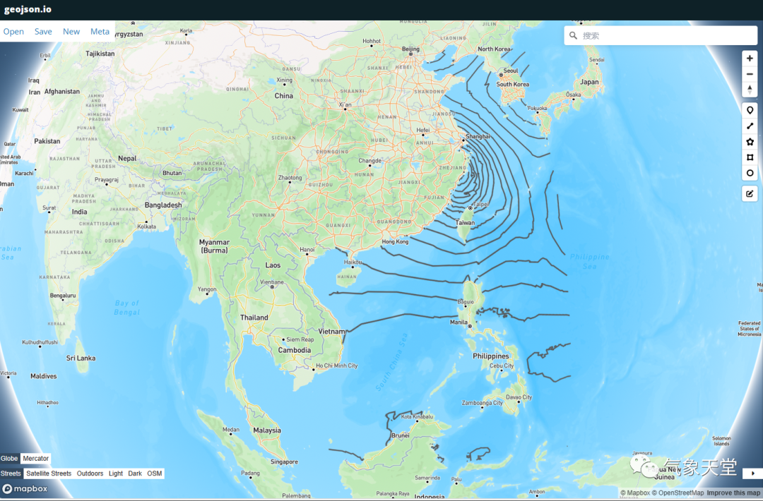
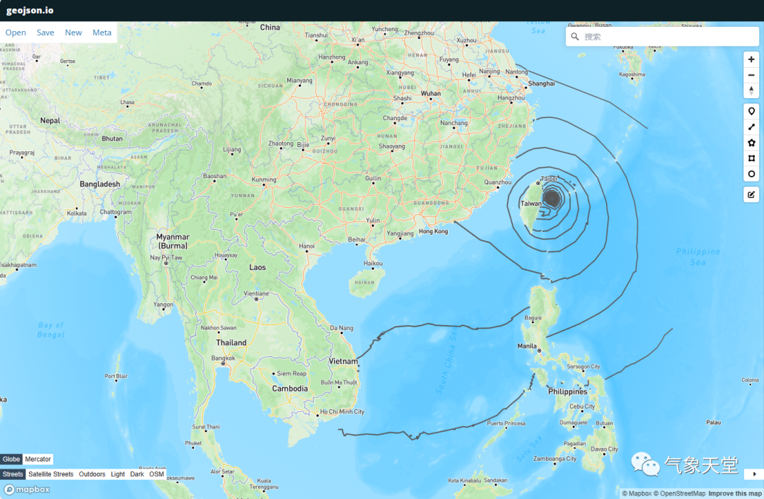
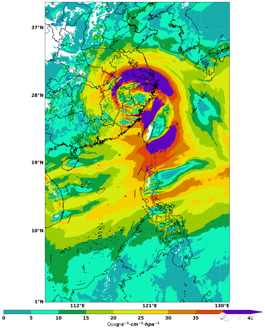
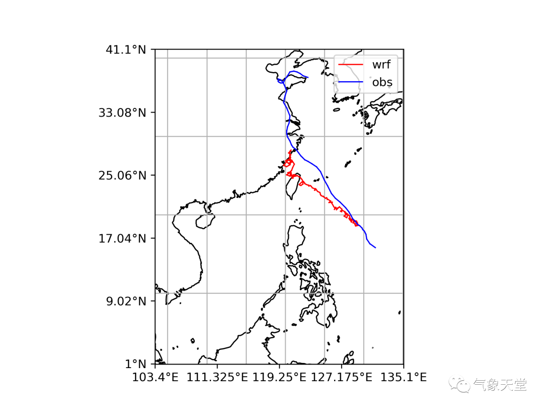
其他的json文件目前还不支持在该网站的显示,需要系统自行适配。台风路径的json文件绘制代码过于冗长,其原理类似,即将最低气压坐标点放入json的字典中(后续将单独讲解一下),并根据10米最大风速规则添加上台风属于'热带低压'、'热带风暴'、'强热带风暴'、'台风'、'强台风'或'超强台风'中的哪一种?另外,还绘制了水汽通量图和台风路径图来验证提取的数据是否准确?

声明:欢迎转载、转发本号原创内容,可留言区留言或者后台联系小编(微信:gavin7675)进行授权。气象学家公众号转载信息旨在传播交流,其内容由作者负责,不代表本号观点。文中部分图片来源于网络,如涉及作品内容、版权和其他问题,请后台联系小编处理。