照相机模型与增强现实

1 针孔照相机模型

1.1 照相机矩阵
1.2 三维点的投影
1.3 照相机矩阵的分解
1.4 照相机中心

2 照相机标定
3 以平面和标记物进行姿态估计
4 增强现实

4.1 PyGame和PyOpenGL
4.2 从照相机矩阵到OpenGL格式
4.5 在图像中放置虚拟物体

本章中，我们将尝试对照相机进行建模，并有效地使用这些模型。在之前的章节里，我们已经讲述了图像到图像这件的映射和变换。为了处理三维图像和平面图像之间的映射，我们需要在映射中加入部分照相机产生图像过程的投影特性。本章中我们将会讲述如何确定照相机的参数，以及在具体应用中，如增强现实，如何使用图像间的投影变换，

1 针孔照相机模型

针孔照相机模型（有时称为射影照相机模型）是计算机视觉中广泛使用的照相机模型。对于大多数应用来说，针孔照相机模型简单，并且具有足够的精准度。这个名字来源于一种类似暗箱机的照相机。该照相机从一个小孔采集射到暗箱内部的光线。在光线投影到图像平面之前，从唯一一个点经过，也就是照相机中心C。在这里插入图片描述
由图像坐标轴和三维坐标系中的x轴和y轴对齐平行的假设，我们可以得出针孔照相机的投影性质。照相机的光学坐标轴和z轴一致，该投影几何一颗简化成相似三角形。在投影之前通过旋转和平移变换，对该坐标系加入三维点，会出现完整的投影变换。

在针孔照相机中，三维点X投影为图像点x（两个点都是用齐次坐标表示的），如下所示： $encoding="application/x-tex">\lambda x=PX</annotation></semantics></math>$ 这里，3×4的矩阵P为照相机矩阵（或投影矩阵）。注意，在齐次坐标系中，三维点X的坐标由4个元素组成，X=[X,Y,Z,W]。这里的标量λ是三维点的逆深度。如果我们打算在齐次坐标中将最后一个数值归一化为1，那么就会使用到它。

1.1 照相机矩阵

照相机矩阵可以分解为： $P = K [R ∣ t]$ 其中，R是描述照相机方向的旋转矩阵，t是描述照相机中心位置的三维平移向量，内标定矩阵K描述照相机的投影性质。

标定矩阵仅和照相机自身的情况相关，通常情况下可以写成： $\begin{bmatrix}\alpha f & s & c_x \\ 0 & f & c_y \\ 0 & 0& 1 \end{bmatrix}</annotation></semantics></math>$ 图像平面和照相机中心间的距离为焦距f。当像素数组在传感器上偏斜的时候，需要用到倾斜参数s。在大多数情况下，s可以设置成0.也就是说： $\begin{bmatrix} f_x & 0 & c_x \\ 0 & f_y & c_y \\ 0 & 0& 1 \end{bmatrix}</annotation></semantics></math>$ 这里，我们使用了另外的记号f _x 和f _y ，两者关系为f _x =αf _y 。

纵横比例参数α是在像素元素非正方形的情况下使用的。通常情况下，我们还可以默认设置α=1.经过这些假设，标定矩阵变为： $\begin{bmatrix} f & 0 & c_x \\ 0 & f & c_y \\ 0 & 0& 1 \end{bmatrix}</annotation></semantics></math>$ 除焦距之外，标定矩阵中剩余的唯一参数为光心（有时称为主点）的坐标c=[c _x ,c _y ]，也就是光线坐标轴和图像平面的交点。因为光心通常在图像的中心，并且图像的坐标是从左上角开始计算的，所以光心的坐标常接近于图像宽度和高度的一半。特别强调一点，这这个例子中，唯一未知的变量是焦距f。

1.2 三维点的投影

下面来创建照相机类，用来处理我们对照相机和投影建模所需要的全部操作：

from scipy import linalg
from pylab import  *

class Camera(object):
    """表示针孔照相机的类"""

    def __init__(self, P):
        """初始化 P = K[R|t] 照相机模型"""
        self.P = P
        self.K = None   # 标定矩阵
        self.R = None   # 旋转
        self.t = None   # 平移
        self.c = None   # 照相机中心

    def project(self, X):
        """X（4×n的数组）的投影点，并进行坐标归一化"""
        x = dot(self.P, X)
        for i in range(3):
            x[i] /= x[2]
        return x

    def rotation_matrix(a):
        """创建一个用于围绕向量a轴旋转的三维旋转矩阵"""
        R = eye(4)
        R[:3,:3] = linalg.expm([0,-a[2],a[1]],[a[2],0,-a[0]],[-a[1],a[0],0])
        return R

1.3 照相机矩阵的分解

如果给定方程（1.1节中）所示的照相机矩阵P，我们需要恢复内参数K以及照相机的位置t和姿势R。矩阵分块操作称为因子分解。这里，我们将使用一种矩阵因子分解的方法，称为RQ因子分解。

将下面的方法添加到Carmera类中：

    def factor(self):
        """将照相机矩阵分解为 K,R,t,其中, R=K[R|t]"""

        # 分解前3×3的部分
        K,R = linalg.rq(self.P[:,:3])

        # 将K的对角线元素设为正值
        T = diag(sign(diag(K)))
        if linalg.det(T) < 0:
            T[1,1] *= -1
        self.K = dot(K,T)
        self.R = dot(T,R)   # T的逆矩阵为其自身
        self.t = dot(linalg.inv(self.K), self.P[:


    
,3])
        
        return self.K, self.R, self.t

RQ因子分解的结果并不是唯一的。在该因子分解中，分解的结果存在符号二义性。由于我们需要限制旋转矩阵R为正定的（否则，旋转坐标轴即可），所以如果需要，我们可以在求解到的结果中加入变换T来改变符号。

在示例照相机上运行下面的代码，观察照相机矩阵分解的效果：

if __name__=='__main__':

    K = array([[1000,0,500],[0,1000,300],[0,0,1]])
    tmp = Camera.rotation_matrix([0,0,1])[:3,:3]
    Rt = hstack((tmp,array([[50],[40],[30]])))
    cam = Camera(dot(K,Rt))

    print(K,Rt)
    print(cam.factor())

输出：
在这里插入图片描述

1.4 照相机中心

给定照相机投影矩阵P，我们可以计算出空间上照相机的所在位置。照相机的中心C，是一个三维点，满足约束PC=0。对于投影矩阵为P=K[R|t]的照相机，有： $K [R ∣ t] C = (adsbygoogle = window.adsbygoogle || []).push({}); K R C + K t = 0$ 照相机的中心可以由下述式子来计算： $encoding="application/x-tex">C=-R^Tt</annotation></semantics></math>$ 注意，如预期一样，照相机的中心和内标定矩阵K无关。

下面的代码可以按照上面公式计算照相机的中心。将其添加到Camera类中，该方法会返回照相机的中心：

    def center(self):
        """计算并返回照相机的中心"""
        if self.c is not None:
            return self.c
        else:
            # 通过因子分解计算c
            self.factor()
            self.c = -dot(self.R.T, self.t)
            return self.c

2 照相机标定

标定照相机是指计算出该照相机的内参数。在我们的例子里，是指计算矩阵K。如果你的应用要求高精度，那么可以扩展该照相机模型，使其包含径向畸变和其他条件。对于大多数应用来说，我们在1.1节中s=0的K公式中的简单照相机模型已经足够。标定照相机的标准方法，拍摄多幅平面期盼模型的图像，然后进行处理计算。

这里我们将要介绍一个简单的照相机标定的方法。大多数参数可以使用基本的假设来设定（正方形垂直的像素，光心位于图像中心），比较难处理的是获得正确的焦距。对于这种标定方法，需要准备一个平面矩形的标定物体（一个书本即可）、用于测量的卷尺和直尺，以及一个平面。下面是具体操作步骤：

1）测量你选定矩形标定物体的边长dX 和 dY；
2）将照相机和标定物体放置在平面上，使得照相机的背面和标定物体平行，同时物体位于3）照相机图像视图的中心，你可能需要调整照相机或者物体来获得良好的对齐效果；
4）测量标定物体到照相机的距离 dZ；
5）拍摄一副图像来检验该设置是否正确，即标定物体的边要和图像的行和列对齐；
6）使用像素数来测量标定物体图像的宽度和高度 dx和 dy

3 以平面和标记物进行姿态估计

在第三章中，我们学习了如何从平面间估计单应性矩阵。如果图像中包含平面状的标记物体，并且已经对照相机进行了标定，那么我们可以计算出照相机的姿态（旋转和平移）。这里的标记物体可以为对任何平坦的物体。

我们使用一个例子来演示如何进行姿态估计。我们使用下面的代码来提取两幅图像的SIFT特征，然后使用RANSAC算法稳健地估计单应性矩阵：

# 计算特征
    sift.process_image('D:\\123\图像处理\Image Processing\Image Processing\Chapter 4\\book_frontal.JPG','im0.sift')
    l0, d0 = sift.read_features_from_file('im0.sift')

    sift.process_image('D:\\123\图像处理\Image Processing\Image Processing\Chapter 4\\book_perspective.JPG','im1.sift')
    l1, d1 = sift.read_features_from_file('im1.sift')

    # 匹配特征，并计算单应性矩阵


    

    matches = sift.match_twosided(d0, d1)
    ndx = matches.nonzero()[0]
    fp = homography.make_homog(l0[ndx,:2].T)
    ndx2 = [int(matches[i]) for i in ndx]
    tp = homography.make_homog(l1[ndx2,:2].T)

    model = homography.RansacModel()
    H = homography.H_from_ransac(fp,tp,model)

现在我们得到了单应性矩阵。该单应性矩阵将一幅图像中标记物（在这个例子中，标记物是指书本）上的点映射到另一幅图像中的对应点。下面我们定义相应的三维坐标系，是标记物在X-Y平面上（Z=0），原点在标记物的某位置上。

为了检验单应性矩阵结果的正确性，我们需要将一些简单的三维物体放置在标记物上，这里我们使用一个立方体。你可以使用下面的函数产生立方体上的点：

def cube_points(c, wid):
    """ Creates a list of points for plotting
        a cube with plot. (the first 5 points are
        the bottom square, some sides repeated). """
    p = []
    # bottom
    p.append([c[0] - wid, c[1] - wid, c[2] - wid])
    p.append([c[0] - wid, c[1] + wid, c[2] - wid])
    p.append([c[0] + wid, c[1] + wid, c[2] - wid])
    p.append([c[0] + wid, c[1] - wid, c[2] - wid])
    p.append([c[0] - wid, c[1] - wid, c[2] - wid])  # same as first to close plot

    # top
    p.append([c[0] - wid, c[1] - wid, c[2] + wid])
    p.append([c[0] - wid, c[1] + wid, c[2] + wid])
    p.append([c[0] + wid, c[1


    
] + wid, c[2] + wid])
    p.append([c[0] + wid, c[1] - wid, c[2] + wid])
    p.append([c[0] - wid, c[1] - wid, c[2] + wid])  # same as first to close plot

    # vertical sides
    p.append([c[0] - wid, c[1] - wid, c[2] + wid])
    p.append([c[0] - wid, c[1] + wid, c[2] + wid])
    p.append([c[0] - wid, c[1] + wid, c[2] - wid])
    p.append([c[0] + wid, c[1] + wid, c[2] - wid])
    p.append([c[0] + wid, c[1] + wid, c[2] + wid])
    p.append([c[0] + wid, c[1] - wid, c[2] + wid])
    p.append([c[0] + wid, c[1] - wid, c[2] - wid])

    return array(p).T
    
def my_calibration(sz):
    row, col = sz
    fx = 2555 * col / 2592
    fy = 2586 * row / 1936
    K = diag([fx, fy, 1])
    K[0, 2] = 0.5 * col
    K[1, 2] = 0.5 * row
    return K

有了单应性矩阵和照相机的标定矩阵，我们现在可以得出两个视图间的相对变换：

#  计算特征
    sift.process_image('D:\\123\图像处理\Image Processing\Image Processing\Chapter 4\\book_frontal.JPG', 'im0.sift')
    l0, d0 = sift.read_features_from_file('im0.sift')

    sift.process_image('D:\\123\图像处理\Image Processing\Image Processing\Chapter 4\\book_perspective.JPG', 'im1.sift')
    l1, d1 = sift.read_features_from_file('im1.sift')

    #  匹配特征并计算单应性矩阵
    matches = sift.match_twosided(d0, d1)
    ndx = matches.nonzero()[0]
    fp = homography.make_homog(l0[ndx, :2].T)
    ndx2 = [int(matches[i]) for i in ndx]
    tp = homography.make_homog(l1[ndx2, :2].T)

    model = homography.RansacModel()
    H, inliers = homography.H_from_ransac(fp, tp, model)

    # 计算照相机标定矩阵
    K = my_calibration((400, 300))

    # 位于边长为0.2 z=0平面的三维点
    box = cube_points([0, 0, 0.1], 0.1)

    # 投影第一幅图像上底部的正方形
    cam1 = camera.Camera(hstack((K, dot(K, array([[0], [0], [-1]])))))
    # 底部正方形上的点
    box_cam1 = cam1.project(homography.make_homog(box[:, :5]))

    # 使用H将点变换到第二幅图像中
    box_trans = homography.normalize(dot(H, box_cam1))

    # 从cam1和H中计算第二个照相机矩阵
    cam2 = camera.Camera(dot(H, cam1.P))
    A = dot(linalg.inv(K), cam2.P[:, :3])
    A = array([A[:, 0], A[:, 1], cross(A[:, 0],


    
 A[:, 1])]).T
    cam2.P[:, :3] = dot(K, A)

    # 使用第二个照相机矩阵投影
    box_cam2 = cam2.project(homography.make_homog(box))

    # plotting
    im0 = array(Image.open('D:\\123\图像处理\Image Processing\Image Processing\Chapter 4\\book_frontal.JPG'))
    im1 = array(Image.open('D:\\123\图像处理\Image Processing\Image Processing\Chapter 4\\book_perspective.JPG'))

    figure()
    imshow(im0)
    plot(box_cam1[0, :], box_cam1[1, :], linewidth=3)
    title('2D projection of bottom square')
    axis('off')

    figure()
    imshow(im1)
    plot(box_trans[0, :], box_trans[1, :], linewidth=3)
    title('2D projection transfered with H')
    axis('off')

    figure()
    imshow(im1)
    plot(box_cam2[0, :], box_cam2[1, :], linewidth=3)
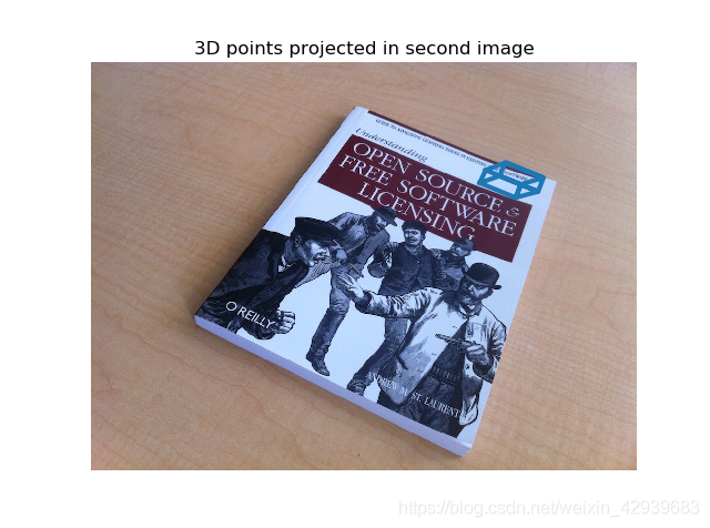
    title('3D points projected in second image')
    axis('off')

    show()

在这里插入图片描述

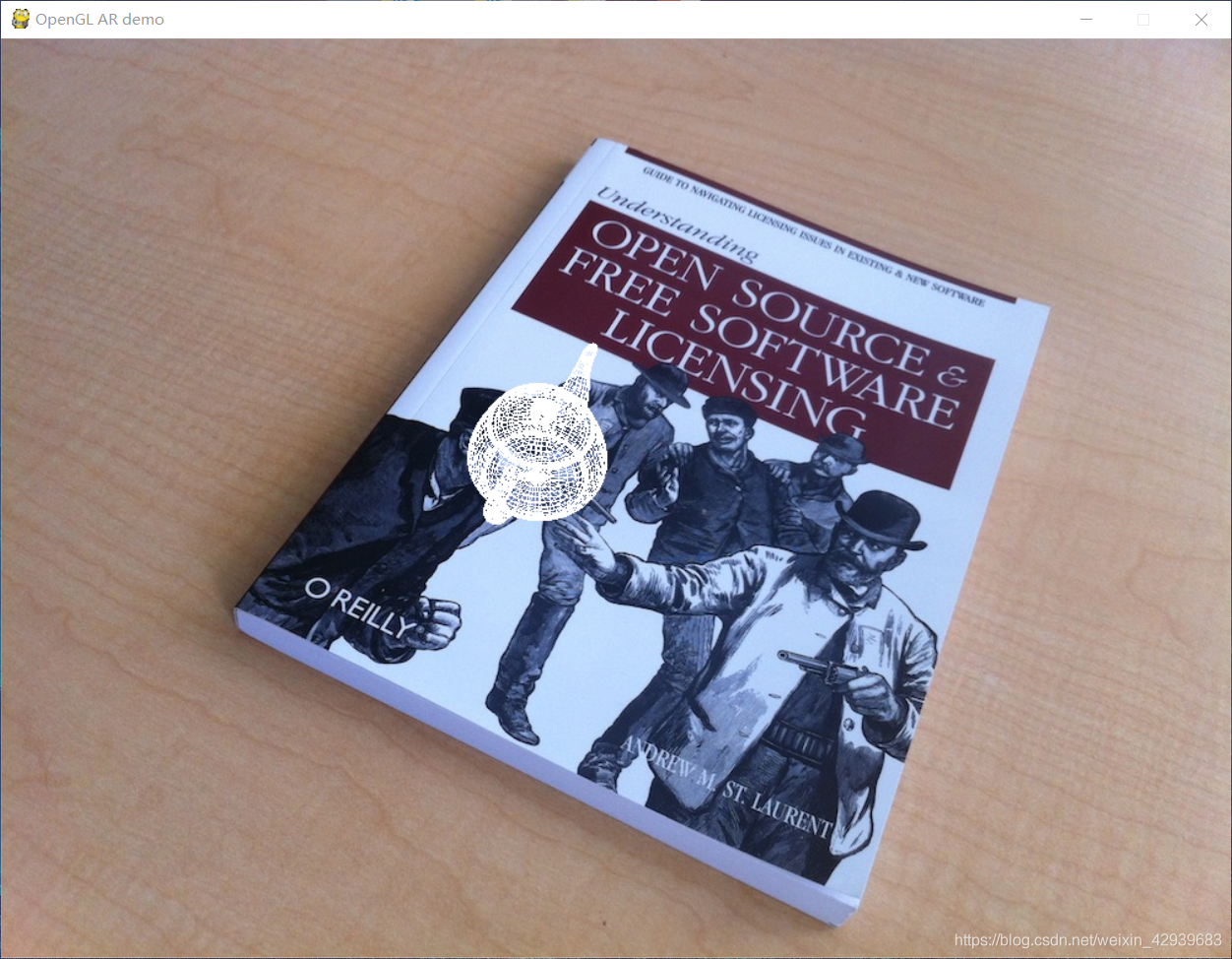
4 增强现实

增强现实（Augmented Reality, AR）是将物体和相应信息放置在图像数据上的一系列操作的总称。最经典的例子是放置一个三维计算机图形学模型，使其看起来属于该场景；如果在视频中，该模型会随着照相机的运动很自然地移动。如上一届所示，给定一幅带有标记平面的图像，我们能够计算出照相机的位置和姿态，使用这些信息来放置计算机图形学模型，能够正确表示它们。在本章的最后一节，我们将介绍如何建立一个简单的增强现实例子。其中，我们会用到两个工具包：PyGame和PyOpenGL。

4.1 PyGame和PyOpenGL

安装PyGame




    
pip install pygame

安装PyOpenGL

pip install PyOpenGL-3.1.5-cp37-cp37m-win_amd64.whl
pip install PyOpenGL_accelerate-3.1.5-cp37-cp37m-win_amd64.whl

测试：

from OpenGL.GL import *
from OpenGL.GLU import *
from OpenGL.GLUT import *


def drawFunc():
    glClear(GL_COLOR_BUFFER_BIT)
    # glRotatef(1, 0, 1, 0)
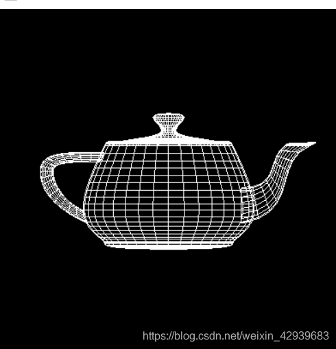
    glutWireTeapot(0.5)
    glFlush()


glutInit()
glutInitDisplayMode(GLUT_SINGLE | GLUT_RGBA)
glutInitWindowSize(400, 400)
# 参数为b类型而不是string
glutCreateWindow(b"First")
glutDisplayFunc(drawFunc)
# glutIdleFunc(drawFunc)
glutMainLoop()

在这里插入图片描述

4.2 从照相机矩阵到OpenGL格式

OpenGL 使用4×4 的矩阵来表示变换（包括三维变换和投影）。这和我们使用的 3×4 照相机矩阵略有差别。但是，照相机与场景的变换分成了两个矩阵，GL_PROJECTION 矩阵和GL_MODELVIEW 矩阵GL_PROJECTION 矩阵处理图像成像的性质，等价于我们的内标定矩阵 K。GL_MODELVIEW 矩阵处理物体和照相机之间的三维变换关系，对应于我们照相机矩阵中的R 和 t 部分。一个不同之处是，假设照相机为坐标系的中心，GL_MODELVIEW 矩阵实际上包含了将物体放置在照相机前面的变换。

假设我们已经获得了标定好的照相机，即已知标定矩阵 K，下面的函数可以将照相机参数转换为 OpenGL 中的投影矩阵：

def set_projection_from_camera(K):
    """从照相机标定矩阵中获得视图"""

    glMatrixMode(GL_PROJECTION)
    glLoadIdentity()

    fx = K[0,0]
    fy = K[1,1]
    fovy = 2 * arctan(0.5*height / fy) * 180 / pi
    aspect = (width*fy) / (height * fx)

    # 定义近的和圆的裁剪平面
    near = 0.1
    far = 100.0
    gluPerspective(fovy, aspect, near, far)
    glViewport(0, 0, width, height)

第一个函数 glMatrixMode() 将工作矩阵设置为 GL_PROJECTION，接下来的命令会修改这个矩阵 1。然后，glLoadIdentity() 函数将该矩阵设置为单位矩阵，这是重置矩阵的一般操作。然后，我们根据图像的高度、照相机的焦距以及纵横比，计算出视图中的垂直场。OpenGL的投影同样具有近距离和远距离的裁剪平面来限制场景拍摄的深度范围。我们设置近深度为一个小的数值，使得照相机能够包含最近的物体，而远深度设置为一个大的数值。我们使用 GLU 的实用函数 gluPerspective() 来设置投影矩阵，将整个图像定义为视图部分（也就是显示的部分）。和下面的模拟视图函数相似，你可以使用 glLoadMatrixf() 函数的一个选项来定义一个完全的投影矩阵。当简单版本的标定矩阵不够好时，可以使用完全投影矩阵。

模拟视图矩阵能够表示相对的旋转和平移，该变换将该物体放置在照相机前（效果是照相机在原点上）。模拟视图矩阵是个典型的 4×4 矩阵，如下所示： $encoding="application/x-tex">\begin{bmatrix}R & t \\ 0 & 1\end{bmatrix}</annotation></semantics></math>$ 其中，R是旋转矩阵，列向量表示3个坐标轴的方向，t是平移向量。当创建模拟视图矩阵时，旋转矩阵需要包括所有的旋转（物体和坐标系的旋转），可以将单个旋转分量相乘来获得旋转矩阵。

下面的函数实现如何获得移除标定矩阵后3×4针孔照相机矩阵（将P和K ^-1 相乘），并创建一个模拟视图：

def set_modelview_from_camera(Rt):
    """从照相机姿态中获得模拟视图矩阵"""

    glMatrixMode(GL_MODELVIEW)
    glLoadIdentity()
    # 围绕x轴将茶壶旋转90度，使z轴向上
    Rx = np.array([[1, 0, 0], [0, 0, -1], [0, 1, 0]])
    # 获得旋转的最佳逼近
    R = Rt[:, :3]
    U, S, V = np.linalg.svd(R)
    R = np.dot(U, V)
    R[0, :] = -R[0, :]  # 改变x轴的符号
    # 获得平移量
    t = Rt[:, 3]
    # 获得4*4的的模拟视图矩阵
    M = np.eye(4)
    M[


    
:3, :3] = np.dot(R, Rx)
    M[:3, 3] = t
    # 转置并压平以获取列序数值
    M = M.T
    m = M.flatten()
    # 将模拟视图矩阵替换成新的矩阵
    glLoadMatrixf(m)

4.5 在图像中放置虚拟物体

import math
import pickle
import sys
from pylab import *
from OpenGL.GL import *
from OpenGL.GLU import *
from OpenGL.GLUT import *
import pygame, pygame.image
from pygame.locals import *
from PCV.geometry import homography, camera
from PCV.localdescriptors import sift


def cube_points(c, wid):  # 绘制立方体的一各点列表
    """ Creates a list of points for plotting
        a cube with plot. (the first 5 points are
        the bottom square, some sides repeated). """
    p = []
    # 底部
    p.append([c[0] - wid, c[1] - wid, c[2] - wid])
    p.append([c[0] - wid, c[1] + wid, c[2] - wid])
    p.append([c[0] + wid, c[1] + wid, c[2] - wid])
    p.append([c[0] + wid, c[1] - wid, c[2] - wid])
    p.append([c[0] - wid, c[1] - wid, c[2] - wid])  # 和第一个相同

    # 顶部
    p.append([c[0] - wid, c[1] - wid, c[2] + wid])
    p.append([c[0] - wid, c[1] + wid,


    
 c[2] + wid])
    p.append([c[0] + wid, c[1] + wid, c[2] + wid])
    p.append([c[0] + wid, c[1] - wid, c[2] + wid])
    p.append([c[0] - wid, c[1] - wid, c[2] + wid])  # 和第一个相同

    # 竖直边
    p.append([c[0] - wid, c[1] - wid, c[2] + wid])
    p.append([c[0] - wid, c[1] + wid, c[2] + wid])
    p.append([c[0] - wid, c[1] + wid, c[2] - wid])
    p.append([c[0] + wid, c[1] + wid, c[2] - wid])
    p.append([c[0] + wid, c[1] + wid, c[2] + wid])
    p.append([c[0] + wid, c[1] - wid, c[2] + wid])
    p.append([c[0] + wid, c[1] - wid, c[2] - wid])

    return array(p).T


def my_calibration(sz):
    row, col = sz
    fx = 2555 * col / 2592
    fy = 2586 * row / 1936
    K = diag([fx, fy, 1])
    K[0, 2] = 0.5 * col
    K[1, 2] = 0.5 * row
    return K


def set_projection_from_camera


    
(K):  # 获取视图
    glMatrixMode(GL_PROJECTION)
    glLoadIdentity()
    fx = K[0, 0]
    fy = K[1, 1]
    fovy = 2 * math.atan(0.5 * height / fy) * 180 / math.pi
    aspect = (width * fy) / (height * fx)
    # 定义近和远的剪裁平面
    near = 0.1
    far = 100.0
    # 设定透视
    gluPerspective(fovy, aspect, near, far)
    glViewport(0, 0, width, height)


def set_modelview_from_camera(Rt):  # 获取矩阵
    glMatrixMode(GL_MODELVIEW)
    glLoadIdentity()
    # 围绕x轴将茶壶旋转90度，使z轴向上
    Rx = np.array([[1, 0, 0], [0, 0, -1], [0, 1, 0]])
    # 获得旋转的最佳逼近
    R = Rt[:, :3]
    U, S, V = np.linalg.svd(R)
    R = np.dot(U, V)
    R[0, :] = -R[0, :]  # 改变x轴的符号
    # 获得平移量
    t = Rt[:, 3]
    # 获得4*4的的模拟视图矩阵
    M = np.eye(4)
    M[:3, :3] = np.dot(R, Rx)
    M[:3, 3] = t
    # 转置并压平以获取列序数值
    M = M.T
    m = M.flatten()
    # 将模拟视图矩阵替换成新的矩阵
    glLoadMatrixf(m)


def draw_background(imname):
    # 载入背景图像
    bg_image = pygame.image.load(imname).convert()
    bg_data = pygame.image.tostring(bg_image, "RGBX", 1)  # 将图像转为字符串描述
    glMatrixMode(GL_MODELVIEW)  # 将当前矩阵指定为投影矩阵
    glLoadIdentity()  # 把矩阵设为单位矩阵

    glClear(GL_COLOR_BUFFER_BIT | GL_DEPTH_BUFFER_BIT)  # 清楚颜色、深度缓冲
    glEnable(GL_TEXTURE_2D)  # 纹理映射
    glBindTexture(GL_TEXTURE_2D, glGenTextures(1))
    glTexImage2D(GL_TEXTURE_2D, 0, GL_RGBA, width, height, 0, GL_RGBA, GL_UNSIGNED_BYTE, bg_data)


    

    glTexParameterf(GL_TEXTURE_2D, GL_TEXTURE_MAG_FILTER, GL_NEAREST)
    glTexParameterf(GL_TEXTURE_2D, GL_TEXTURE_MIN_FILTER, GL_NEAREST)
    # 绑定纹理
    glBegin(GL_QUADS)
    glTexCoord2f(0.0, 0.0);
    glVertex3f(-1.0, -1.0, -1.0)
    glTexCoord2f(1.0, 0.0);
    glVertex3f(1.0, -1.0, -1.0)
    glTexCoord2f(1.0, 1.0);
    glVertex3f(1.0, 1.0, -1.0)
    glTexCoord2f(0.0, 1.0);
    glVertex3f(-1.0, 1.0, -1.0)
    glEnd()
    glDeleteTextures(1)  # 清除纹理


def draw_teapot(size):  # 红色茶壶
    glEnable(GL_LIGHTING)
    glEnable(GL_LIGHT0)
    glEnable(GL_DEPTH_TEST)
    glClear(GL_DEPTH_BUFFER_BIT)
    # 绘制红色茶壶
    glMaterialfv(GL_FRONT, GL_AMBIENT, [0, 0, 0, 0])
    glMaterialfv(GL_FRONT, GL_DIFFUSE, [0.5, 0.0, 0.0, 0.0])
    glMaterialfv(GL_FRONT, GL_SPECULAR, [0.7, 0.6, 0.6, 0.0])
    glMaterialf(GL_FRONT, GL_SHININESS, 0.25 * 128.0)
    glutSolidTeapot(size)


def drawFunc(size):  # 白色茶壶
    glRotatef(0.5, 5, 5, 0)  # (角度,x,y,z)
    glutWireTeapot(size)
    # 刷新显示
    glFlush()


width, height = 1000, 747


def setup():  # 设置窗口和pygame环境
    pygame.init()
    pygame.display.set_mode((width, height), OPENGL | DOUBLEBUF)
    pygame.display.set_caption("OpenGL AR demo")


# 计算特征
sift.process_image('D:\\123\图像处理\Image Processing\Image Processing\Chapter 4\\book_frontal.JPG', 'im0.sift')
l0, d0 = sift.read_features_from_file('im0.sift')

sift.process_image('D:\\123\图像处理\Image Processing\Image Processing\Chapter 4\\book_perspective.JPG','im1.sift')
l1, d1 = sift.read_features_from_file('im1.sift')

# 匹配特征，计算单应性矩阵
matches = sift.match_twosided(d0, d1)
ndx = matches.nonzero()[


    
0]
fp = homography.make_homog(l0[ndx, :2].T)
ndx2 = [int(matches[i]) for i in ndx]
tp = homography.make_homog(l1[ndx2, :2].T)

model = homography.RansacModel()
H, inliers = homography.H_from_ransac(fp, tp, model)

# 计算照相机标定矩阵
K = my_calibration((747, 1000))
# 位于边长为0.2，z=0平面上的三维点
box = cube_points([0, 0, 0.1], 0.1)

# 投影第一幅图下个上底部的正方形
cam1 = camera.Camera(hstack((K, dot(K, array([[0], [0], [-1]])))))
# 底部正方形上的点
box_cam1 = cam1.project(homography.make_homog(box[:, :5]))

# 使用H将点变换到第二幅图像中
box_trans = homography.normalize(dot(H, box_cam1))

# 从cam1和H中计算第二个照相机矩阵
cam2 = camera.Camera(dot(H, cam1.P))
A = dot(linalg.inv(K), cam2.P[:, :3])
A = array([A[:, 0], A[:, 1], cross(A[:, 0], A[:, 1])]).T
cam2.P[:, :3] = dot(K, A)
# 使用第二个照相机矩阵投影
box_cam2 = cam2.project(homography.make_homog(box))

Rt = dot(linalg.inv(K), cam2.P)
setup()
draw_background("D:\\123\图像处理\Image Processing\Image Processing\Chapter 4\\book_perspective.bmp")
set_projection_from_camera(K)
set_modelview_from_camera(Rt)

#draw_teapot(0.05)  # 显示红色茶壶
drawFunc(0.05)  # 显示白色空心茶壶
pygame.display.flip()
while True:
    for event in pygame.event.get():
        if event.type == pygame.QUIT:
            sys.exit


    
()

在这里插入图片描述

Python计算机视觉编程第四章 照相机模型与增强现实

照相机模型与增强现实

1 针孔照相机模型

1.1 照相机矩阵

(adsbygoogle = window.adsbygoogle || []).push({}); 1.2 三维点的投影

1.3 照相机矩阵的分解

1.4 照相机中心

2 照相机标定

3 以平面和标记物进行姿态估计

4 增强现实

4.1 PyGame和PyOpenGL

4.2 从照相机矩阵到OpenGL格式

4.5 在图像中放置虚拟物体

Python计算机视觉编程第四章照相机模型与增强现实

1.2 三维点的投影