读入数据
# 导入包
import numpy as np
import pandas as pd
import matplotlib.pyplot as plt
import seaborn as sns
from pyecharts.charts import Bar, Pie, Page
from pyecharts import options as opts
from
pyecharts.globals import SymbolType, WarningType
WarningType.ShowWarning = False
plt.rcParams['font.sans-serif'] = ['SimHei']  # 用来正常显示中文标签
plt.rcParams['axes.unicode_minus'] = False  # 用来正常显示负号
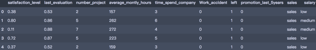
# 读入数据
df = pd.read_csv('HR_comma_sep.csv')
df.head()
<class 'pandas.core.frame.DataFrame'>
RangeIndex: 14999 entries, 0 to 14998
Data columns (total 10 columns):
# Column Non-Null Count Dtype
--- ------ -------------- -----
0 satisfaction_level 14999 non-null float64
1 last_evaluation 14999 non-null float64
2 number_project 14999 non-null int64
3 average_montly_hours 14999 non-null int64
4 time_spend_company 14999 non-null int64
5 Work_accident 14999 non-null int64
6
left 14999 non-null int64
7 promotion_last_5years 14999 non-null int64
8 sales 14999 non-null object
9 salary 14999 non-null object
dtypes: float64(2), int64(6), object(2)
memory usage: 1.1+ MB
# 查看缺失值
print(df.isnull().any().sum())
可以发现,数据质量良好,没有缺失数据。
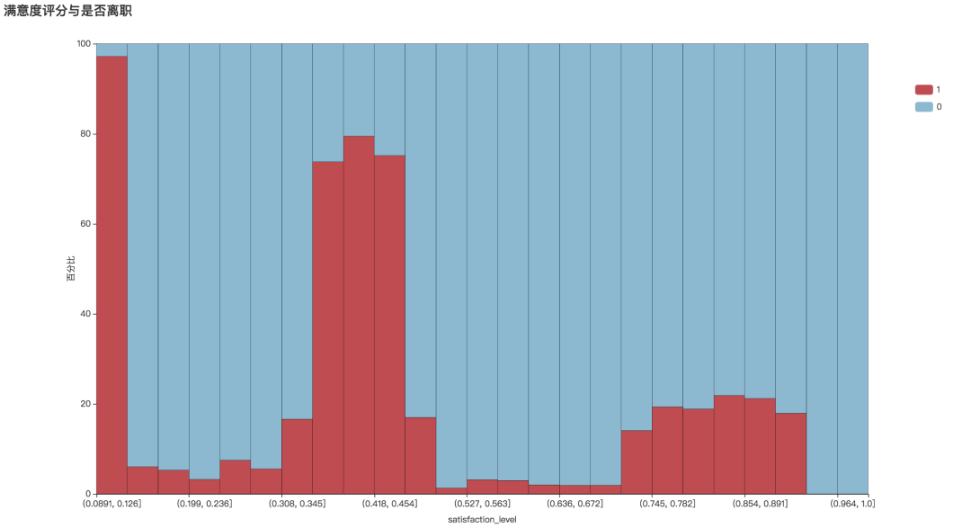
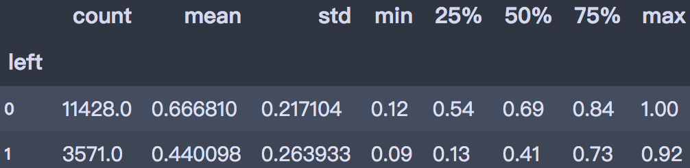
从直方图可以看出,离职员工的满意度评分明显偏低,平均值为0.44。满意度低于0.126分的离职率为97.2%。可见提升员工满意度可以有效防止人员流失。
df.groupby('left')['satisfaction_level'].describe()
def draw_numeric_graph(x_series, y_series, title):
    # 产生数据
    sat_cut = pd.cut(x_series, bins=25)
    cross_table = round(pd.crosstab(sat_cut, y_series, normalize='index'),4)*100
    x_data = cross_table.index.astype('str').tolist()
    y_data1 = cross_table[cross_table.columns[1]].values.tolist()
    y_data2 = cross_table[cross_table.columns[0]].values.tolist()

    # 条形图
    bar = Bar(init_opts=opts.InitOpts(width='1350px', height='750px'))
    bar.add_xaxis(x_data)
    bar.add_yaxis(str(cross_table.columns[1]), y_data1, stack='stack1', category_gap='0%')
    bar.add_yaxis(str(cross_table.columns[0]), y_data2, stack='stack1', category_gap='0%')
    bar.set_global_opts(title_opts=opts.TitleOpts(title),
                        xaxis_opts=opts.AxisOpts(name=x_series.name, name_location='middle', name_gap=30),
                        yaxis_opts=opts.AxisOpts(name='百分比', name_location='middle', name_gap=30, min_=0, max_=100),
                        legend_opts=opts.LegendOpts(orient='vertical', pos_top='15%', pos_right='2%'))
    bar.set_series_opts(label_opts=opts.LabelOpts(is_show=False),
                        itemstyle_opts=opts.ItemStyleOpts(border_color='black', border_width=0.3))
    bar.set_colors(['#BF4C51', '#8CB9D0'])

    return bar
bar1 = draw_numeric_graph(df['satisfaction_level'], df['left'], title='满意度评分与是否离职')
bar1.render()
建模分析
我们使用决策树和随机森林进行模型建置,首先导入所需包:
from sklearn.model_selection import train_test_split, GridSearchCV
from sklearn.tree import DecisionTreeClassifier
from sklearn.ensemble import RandomForestClassifier
from sklearn.metrics import classification_report, f1_score, roc_curve, plot_roc_curve
然后划分训练集和测试集,采用分层抽样方法划分80%数据为训练集,20%数据为测试集。
x = df_dummies.drop('left', axis=1)
y = df_dummies['left']

X_train, X_test, y_train, y_test = train_test_split(x, y, test_size=0.2, stratify=y, random_state=2020)
print(X_train.shape, X_test.shape, y_train.shape, y_test.shape)
我们使用决策树进行建模,设置特征选择标准为gini,树的深度为5。输出分类的评估报告:
# 训练模型
clf = DecisionTreeClassifier(criterion='gini', max_depth=5, random_state=25)
clf.fit(X_train, y_train)
train_pred = clf.predict(X_train)
test_pred = clf.predict(X_test)
print('训练集:', classification_report(y_train, train_pred))
print('-' * 60)
print('测试集:', classification_report(y_test, test_pred))
训练集:               precision    recall  f1-score   support

           0       0.98      0.99      0.98      9142
           1       0.97      0.93      0.95      2857

    accuracy                           0.98     11999
   macro avg       0.97      0.96      0.97     11999
weighted avg       0.98      0.98      0.97     11999

------------------------------------------------------------
测试集:               precision    recall  f1-score   support

           0       0.98      0.99      0.98      2286
           1       0.97      0.93      0.95       714

    accuracy                           0.98      3000
   macro avg       0.97      0.96      0.97      3000
weighted avg       0.98      0.98      0.98      3000
假设我们关注的是1类(即离职类)的F1-score,可以看到训练集的分数为0.95,测试集分数为0.95。
# 重要性
imp = pd.DataFrame([*zip(X_train.columns,clf.feature_importances_)], columns=['vars',
'importance'])
imp.sort_values('importance', ascending=False)
imp = imp[imp.importance!=0]
imp
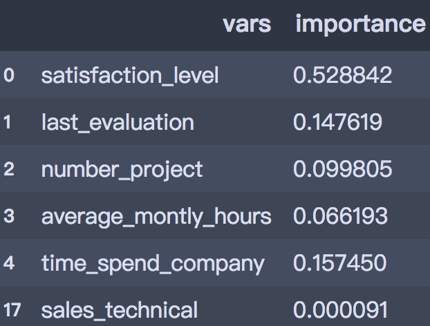
在属性的重要性排序中,员工满意度最高,其次是最新的绩效考核、参与项目数、每月工作时长。
然后使用网格搜索进行参数调优。
parameters = {'splitter':('best','random'),
              'criterion':("gini","entropy"),
              "max_depth":[*range(1, 20)],
             }

clf = DecisionTreeClassifier(random_state=25)
GS = GridSearchCV(clf, parameters, cv=10)
GS.fit(X_train, y_train)

print(GS.best_params_)

print(GS.best_score_)
{'criterion': 'gini', 'max_depth': 15, 'splitter': 'best'}
0.9800813177648042
使用最优的模型重新评估训练集和测试集效果:
train_pred = GS.best_estimator_.predict(X_train)
test_pred = GS.best_estimator_.predict(X_test)

print('训练集:', classification_report(y_train, train_pred))
print('-' * 60)
print('测试集:', classification_report(y_test, test_pred))
训练集: precision recall f1-score support
0 1.00 1.00 1.00 9142
1 1.00 0.99 0.99 2857
accuracy 1.00 11999
macro avg 1.00 0.99 1.00 11999
weighted avg 1.00 1.00 1.00 11999
------------------------------------------------------------
测试集: precision recall f1-score support
0 0.99 0.98 0.99 2286
1 0.95 0.97 0.96 714
accuracy 0.98 3000
macro avg 0.97 0.98 0.97 3000
weighted avg 0.98 0.98 0.98 3000
可见在最优模型下模型效果有较大提升,1类的F1-score训练集的分数为0.99,测试集分数为0.96。
下面使用集成算法随机森林进行模型建置,并调整max_depth参数。
rf_model = RandomForestClassifier(n_estimators=1000, oob_score=True, n_jobs=-1,
                                  random_state=0)
parameters = {'max_depth': np.arange(3, 17, 1) }
GS = GridSearchCV(rf_model, param_grid=parameters, cv=10)
GS.fit(X_train, y_train)

print(GS.best_params_)
print(GS.best_score_)
{'max_depth': 16}
0.988582151793161
train_pred = GS.best_estimator_.predict(X_train)
test_pred = GS.best_estimator_.predict(X_test)

print('训练集:', classification_report(y_train, train_pred))
print('-' * 60)
print('测试集:', classification_report(y_test, test_pred))
训练集: precision recall f1-score support
0 1.00 1.00 1.00 9142
1 1.00 0.99 0.99 2857
accuracy 1.00 11999
macro avg 1.00 1.00 1.00 11999
weighted avg 1.00 1.00 1.00 11999
------------------------------------------------------------
测试集: precision recall f1-score support
0 0.99 1.00 0.99 2286
1 0.99 0.97 0.98 714
accuracy 0.99
3000
macro avg 0.99 0.99 0.99 3000
weighted avg 0.99 0.99 0.99 3000
可以看到在调优之后的随机森林模型中,1类的F1-score训练集的分数为0.99,测试集分数为0.98。
模型后续可优化方向:
以上就是今天的数据分析实例分享了,如果你还想了解其他方面的实战案例,欢迎在评论区给我们留言哦。
本文出品:CDA数据分析师(ID: cdacdacda)


