作者 :Matthew Smith 翻译:张若楠 校对:吴金笛本文约6700字,建议阅读10分钟
本文利用Iris数据集训练了多组机器学习模型,并通过预测大量的拟合数据绘制出了每个模型的决策边界。我使用Iris数据集训练了一系列机器学习模型,从数据中的极端值合成了新数据点,并测试了许多机器学习模型来绘制出决策边界,这些模型可根据这些边界在2D空间中进行预测,这对于阐明目的和了解不同机器学习模型如何进行预测会很有帮助。机器学习模型可以胜过传统的计量经济学模型,这并没有什么新奇的,但是作为研究的一部分,我想说明某些模型为什么以及如何进行分类预测。我想展示我的二分类模型所依据的决策边界,也就是展示数据进行分类预测的分区空间。该问题以及代码经过一些调整也能够适用于多分类问题。
首先加载一系列程序包,然后新建一个logistic函数,以便稍后将log-odds转换为logistic概率函数。library(dplyr)library(patchwork)library(ggplot2)library(knitr)library(kableExtra)library(purrr)
library(stringr)library(tidyr)library(xgboost)library(lightgbm)library(keras)library(tidyquant)##################### Pre-define some functions
logit2prob odds prob return(prob)}
我使用的iris数据集包含有关英国统计员Ronald Fisher在1936年收集的3种不同植物变量的信息。该数据集包含4种植物物种的不同特征,这些特征可区分33种不同物种(Setosa,Virginica和Versicolor)。但是,我的问题需要一个二元分类问题,而不是一个多分类问题。在下面的代码中,我导入了iris数据并删除了一种植物物种virginica,以将其从多重分类转变为二元分类问题。data(iris)df % filter(Species != "virginica") %>% mutate(Species = +(Species == "versicolor"))str(df)
## 'data.frame': 100 obs. of 5 variables:## $ Sepal.Length: num 5.1 4.9 4.7 4.6 5 5.4 4.6 5 4.4 4.9 ...## $ Sepal.Width : num 3.5 3 3.2 3.1 3.6 3.9 3.4 3.4 2.9 3.1 ...## $ Petal.Length: num 1.4 1.4 1.3 1.5 1.4 1.7 1.4 1.5 1.4 1.5 ...## $ Petal.Width : num 0.2 0.2 0.2 0.2 0.2 0.4 0.3 0.2 0.2 0.1 ...## $ Species : int 0 0 0 0 0 0 0 0 0 0 ...
我首先采用ggplot来绘制数据,以下储存的ggplot对象中,每个图仅更改x和y变量选择。plt1 % ggplot(aes(x = Sepal.Width, y = Sepal.Length, color = factor(Species))) + geom_point(size = 4) + theme_bw(base_size = 15) + theme(legend.position = "none")plt2 % ggplot(aes(x = Petal.Length, y = Sepal.Length, color = factor(Species))) + geom_point(size = 4) + theme_bw(base_size = 15) + theme(legend.position = "none")
plt3 % ggplot(aes(x = Petal.Width, y = Sepal.Length, color = factor(Species))) + geom_point(size = 4) + theme_bw(base_size = 15) + theme(legend.position = "none")plt3 % ggplot(aes(x = Sepal.Length, y = Sepal.Width, color = factor(Species))) + geom_point(size = 4) + theme_bw(base_size = 15) + theme(legend.position = "none")plt4 % ggplot(aes(x = Petal.Length, y = Sepal.Width, color = factor(Species))) + geom_point(size = 4) + theme_bw(base_size = 15) + theme(legend.position = "none")
plt5 % ggplot(aes(x = Petal.Width, y = Sepal.Width, color = factor(Species))) + geom_point(size = 4) + theme_bw(base_size = 15) + theme(legend.position = "none")plt6 % ggplot(aes(x = Petal.Width, y = Sepal.Length, color = factor(Species))) + geom_point(size = 4) + theme_bw(base_size = 15) + theme(legend.position = "none")
我还使用了新的patchwork 包,使展示ggplot结果变得很容易。下面的代码很直白的绘制了我们的图形(1个顶部图占满了网格空间的长度,2个中等大小的图,另一个单个图以及底部另外2个图)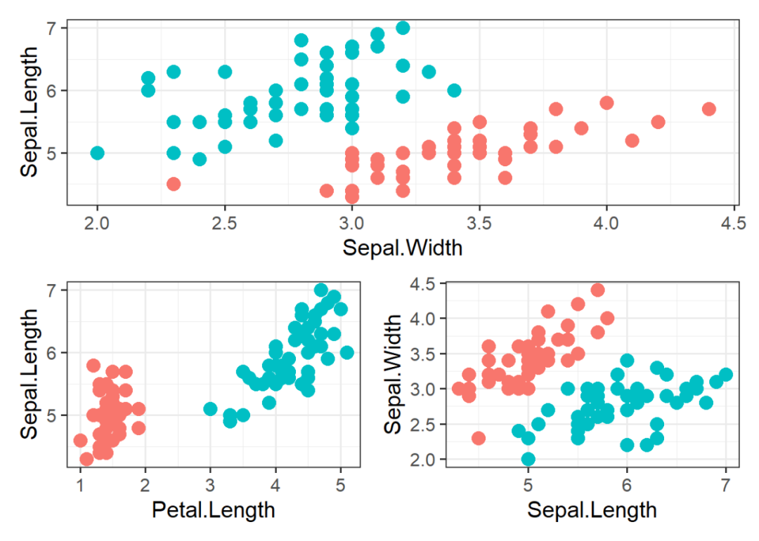
或者,我们可以将绘图重新布置为所需的任何方式,并通过以下方式进行绘图:(plt1 + plt2) / (plt5 + plt6)
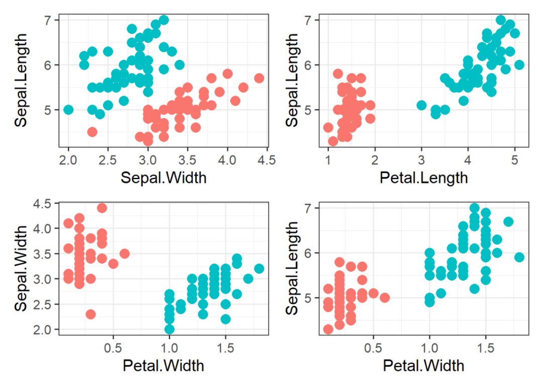
我的目标是建立一种分类算法,以区分这两个植物种类,然后计算决策边界,以便更好地了解模型如何做出此类预测。为了为每个变量组合创建决策边界图,我们需要数据中变量的不同组合。var_combos % filter(!Var1 == Var2)var_combos %>% head() %>% kable(caption = "Variable Combinations", escape = F,, digits = 2) %>%kable_styling(bootstrap_options = c("striped", "hover", "condensed", "responsive"), font_size = 9, fixed_thead = T, full_width = F) %>% scroll_box(width = "100%", height = "200px")
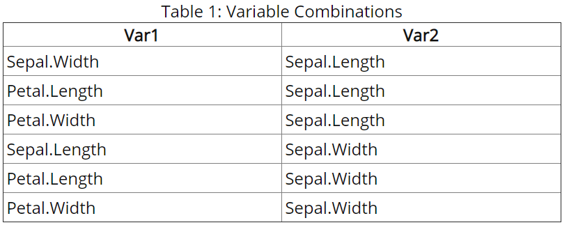
接下来,我将用到以上不同的变量组合来创建列表(每个组合一个列表),并用合成数据(或每个变量组合的最小值到最大值的数据)给列表赋值。这将作为我们的合成测试数据,对其进行预测并建立决策边界。需要注意的是这些图最终将是二维的,因此我们仅在两个变量上训练机器学习模型,但是对于这两个变量的每种组合而言,它们将是取boundary_lists data frame中的前两个变量。
boundary_lists .x = var_combos$Var1, .y = var_combos$Var2, ~select(df, .x, .y) %>% summarise( minX = min(.[[1]], na.rm = TRUE), maxX = max(.[[1]], na.rm = TRUE), minY = min(.[[2]], na.rm = TRUE), maxY = max(.[[2]], na.rm = TRUE) )
) %>% map(., ~tibble( x = seq(.x$minX, .x$maxX, length.out = 200), y = seq(.x$minY, .x$maxY, length.out = 200), ) ) %>% map(., ~tibble( xx = rep(.x$x, each = 200), yy = rep(.x$y, time = 200) ) ) %>% map2(., asplit(var_combos, 1), ~ .x %>% set_names(.y))
boundary_lists %>% map(., ~head(., 4)) %>% head(2)
## [[1]]## # A tibble: 4 x 2## Sepal.Width Sepal.Length## ## 1 2 4.3## 2 2 4.31## 3 2 4.33
## 4 2 4.34#### [[2]]## # A tibble: 4 x 2## Petal.Length Sepal.Length## ## 1 1 4.3## 2 1 4.31## 3 1 4.33## 4 1 4.34
boundary_lists %>% map(., ~head(., 4)) %>% tail(2)
## [[1]]## # A tibble: 4 x 2## Sepal.Width Petal.Width## ## 1 2 0.1 ## 2 2 0.109## 3 2 0.117## 4 2 0.126#### [[2]]## # A tibble: 4 x 2## Petal.Length Petal.Width## ## 1 1 0.1 ## 2 1 0.109
## 3 1 0.117## 4 1 0.126
现在,我们已经建立了测试用模拟数据,我想根据实际观察到的观测值训练模型。我将使用到上面图中的每个数据点训练以下模型:逻辑回归模型
支持向量机+线性核
支持向量机+多项式核
支持向量机 +径向核
支持向量机+sigmoid核
随机森林
默认参数下的XGBoost模型
单层Keras神经网络(带有线性组成)
更深层的Keras神经网络(带有线性组成)
更深一层的Keras神经网络(带有线性组成)
默认参数下的LightGBM模型
旁注:我不是深度学习/ Keras / Tensorflow方面的专家,所以我相信有更好的模型产生更好的决策边界,但是用purrr、map来训练不同的机器学习模型是件很有趣的事。####################################################################################################################################################################### params_lightGBM # objective = "binary",# metric = "auc",# min_data = 1
# )
# To install Light GBM try the following in your RStudio terinal
# git clone --recursive https://github.com/microsoft/LightGBM# cd LightGBM# Rscript build_r.R
models_list % mutate(modeln = str_c('mod', row_number())) %>% pmap(~ {
xname = ..1 yname = ..2 modelname = ..3 df %>% select(Species, xname, yname) %>% group_by(grp = 'grp') %>% nest() %>% mutate(models = map(data, ~{
list( # Logistic Model Model_GLM = { glm(Species ~ ., data = .x, family = binomial(link='logit'))
}, # Support Vector Machine (linear) Model_SVM_Linear = { e1071::svm(Species ~ ., data = .x, type = 'C-classification', kernel = 'linear') }, # Support Vector Machine (polynomial) Model_SVM_Polynomial = { e1071::svm(Species ~ ., data = .x, type = 'C-classification', kernel = 'polynomial') }, # Support Vector Machine (sigmoid) Model_SVM_radial = { e1071::svm(Species ~ ., data = .x, type = 'C-classification', kernel = 'sigmoid') }, # Support Vector Machine (radial) Model_SVM_radial_Sigmoid = { e1071::svm(Species ~ ., data = .x, type = 'C-classification', kernel = 'radial') }, # Random Forest Model_RF = { randomForest::randomForest(formula = as.factor(Species) ~ ., data = .) }, # Extreme Gradient Boosting Model_XGB = {
xgboost( objective = 'binary:logistic', eval_metric = 'auc', data = as.matrix(.x[, 2:3]), label = as.matrix(.x$Species), # binary variable nrounds = 10) }, # Kera Neural Network Model_Keras = { mod % layer_dense(units = 2, activation = 'relu', input_shape = 2) %>% layer_dense(units = 2, activation = 'sigmoid')
mod %>% compile( loss = 'binary_crossentropy', optimizer_sgd(lr = 0.01, momentum = 0.9), metrics = c('accuracy') ) fit(mod, x = as.matrix(.x[, 2:3]), y = to_categorical(.x$Species, 2), epochs = 5,
batch_size = 5, validation_split = 0 ) print(modelname) assign(modelname, mod)
}, # Kera Neural Network Model_Keras_2 = { mod % layer_dense(units = 2, activation = 'relu', input_shape = 2) %>% layer_dense(units = 2, activation = 'linear', input_shape = 2) %>% layer_dense(units = 2, activation = 'sigmoid')
mod %>% compile( loss = 'binary_crossentropy', optimizer_sgd(lr = 0.01, momentum = 0.9), metrics = c('accuracy') ) fit(mod, x = as.matrix(.x[, 2:3]), y = to_categorical(.x$Species, 2), epochs = 5,
batch_size = 5, validation_split = 0 ) print(modelname) assign(modelname, mod)
}, # Kera Neural Network Model_Keras_3 = { mod % layer_dense(units = 2, activation = 'relu', input_shape = 2) %>% layer_dense(units = 2, activation = 'relu', input_shape = 2) %>% layer_dense(units = 2, activation = 'linear', input_shape = 2) %>% layer_dense(units = 2, activation = 'sigmoid')
mod %>% compile( loss = 'binary_crossentropy', optimizer_sgd(lr = 0.01, momentum = 0.9), metrics = c('accuracy') ) fit(mod, x = as.matrix(.x[, 2:3]),
y = to_categorical(.x$Species, 2), epochs = 5, batch_size = 5, validation_split = 0 ) print(modelname) assign(modelname, mod)
},
# LightGBM model Model_LightGBM = { lgb.train( data = lgb.Dataset(data = as.matrix(.x[, 2:3]), label = .x$Species), objective = 'binary', metric = 'auc', min_data = 1 #params = params_lightGBM, #learning_rate = 0.1 ) }
)
}
))
}) %>% map( ., ~unlist(., recursive = FALSE) )
现在我们有了训练好的模型以及预测,我们可以将这些预测重新放回数据中用ggplot进行可视化,然后使用patchwork包进行排版。
plot_data .x = boundary_lists, .y = map( models_predict, ~map(., ~tibble(.) ) ), ~bind_cols(.x, .y))
names(plot_data) plot_data, ~c( paste( colnames(.)[1], "and", colnames(.)[2], sep = "_") )
)
ggplot_lists % map( ., ~select( ., -contains("Model") ) %>% pivot_longer(cols = contains("Prediction"), names_to = "Model", values_to = "Prediction") ) %>% map( .x = ., ~ggplot() + geom_point(aes( x = !!rlang::sym(colnames(.x)[1]), y = !!rlang::sym(colnames(.x)[2]), color = factor(!!rlang::sym(colnames(.x)[4])) ), data = .x) + geom_contour(aes( x = !!rlang::sym(colnames(.x)[1]), y = !!rlang::sym(colnames(.x)[2]), z = !!rlang::sym(colnames(.x)[4]) ), data = .x) + geom_point(aes( x = !!rlang::sym(colnames(.x)[1]), y = !!rlang::sym(colnames(.x)[2]), color = factor(!!rlang::sym(colnames(df)[5])) # this is the status variable
), size = 8, data = df) + geom_point(aes( x = !!rlang::sym(colnames(.x)[1]), y = !!rlang::sym(colnames(.x)[2]) ), size = 8, shape = 1, data = df) + facet_wrap(~Model) + theme_bw(base_size = 25) + theme(legend.position = "none") )
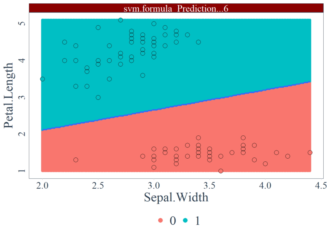
绘制决策边界的所有不同组合。注意:以上的代码在你的console中会运行得更好,当我用代码来编程此博文的时候图像很小。因此,我为模型和变量组合的示例提供了单独的图。我首先需要选择前两列,这是我们的目标变量(Petal.Width,Petal.Length,Sepal.Width和Sepal.Length)。然后,我想在之后随机抽取各列的样本(也就是不同机器学习模型的预测结果)。plot_data_sampled % map( ., ~select( ., -contains("Model") ) %>% select(., c(1:2), sample(colnames(.), 2) ) %>% pivot_longer( cols = contains("Prediction"), names_to = "Model", values_to = "Prediction") )
plot_data_sampled %>% rlist::list.sample(1) %>% map( .x = ., ~ggplot() + geom_point(aes( x = !!rlang::sym(colnames(.x)[1]), y = !!rlang::sym(colnames(.x)[2]), color = factor(!!rlang::sym(colnames(.x)[4])) ), data = .x) + geom_contour(aes( x = !!rlang::sym(colnames(.x)[1]), y = !!rlang::sym(colnames(.x)[2]), z = !!rlang::sym(colnames(.x)[4]) ), data = .x) + geom_point(aes( x = !!rlang::sym(colnames(.x)[1]), y = !!rlang::sym(colnames(.x)[2]), color = factor(!!rlang::sym(colnames(df)[5])) # this is the status variable ), size = 3, data = df) + geom_point(aes( x = !!rlang::sym(colnames(.x)[1]), y = !!rlang::sym(colnames(.x)[2]) ), size = 3, shape = 1, data = df) + facet_wrap(~Model) + #coord_flip() + theme_tq(base_family = "serif") +
theme( #aspect.ratio = 1, axis.line.y = element_blank(), axis.ticks.y = element_blank(), legend.position = "bottom", #legend.title = element_text(size = 20), #legend.text = element_text(size = 10), axis.title = element_text(size = 20), axis.text = element_text(size = "15"), strip.text.x = element_text(size = 15), plot.title = element_text(size = 30, hjust = 0.5), strip.background = element_rect(fill = 'darkred'), panel.background = element_blank(), panel.grid.major = element_blank(), panel.grid.minor = element_blank(), #axis.text.x = element_text(angle = 90), axis.text.y = element_text(angle = 90, hjust = 0.5), #axis.title.x = element_blank() legend.title = element_blank(), legend.text = element_text(size = 20) ) )
## $Sepal.Width_and_Petal.Length## Warning: Row indexes must be between 0 and the number of rows (0). Use `NA` as row index to obtain a row full of `NA` values.## This warning is displayed once per session.
## $Sepal.Width_and_Sepal.Length
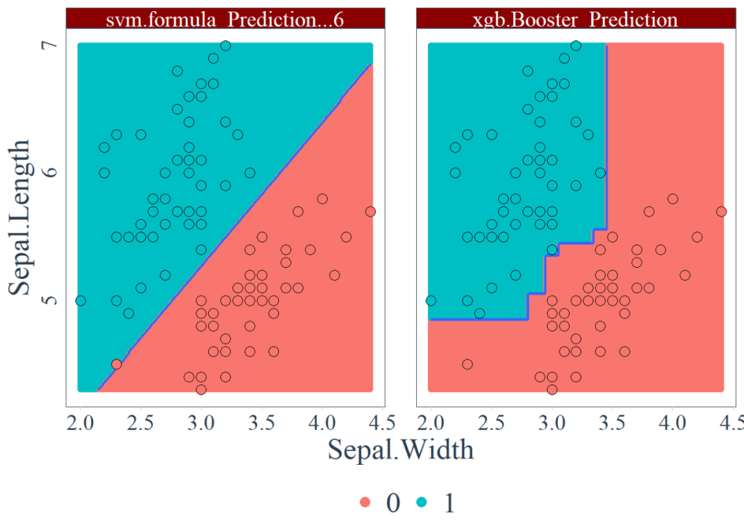
## $Sepal.Width_and_Sepal.Length
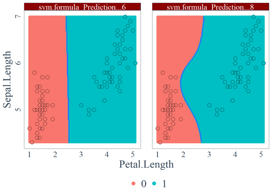
## $Petal.Length_and_Sepal.Length
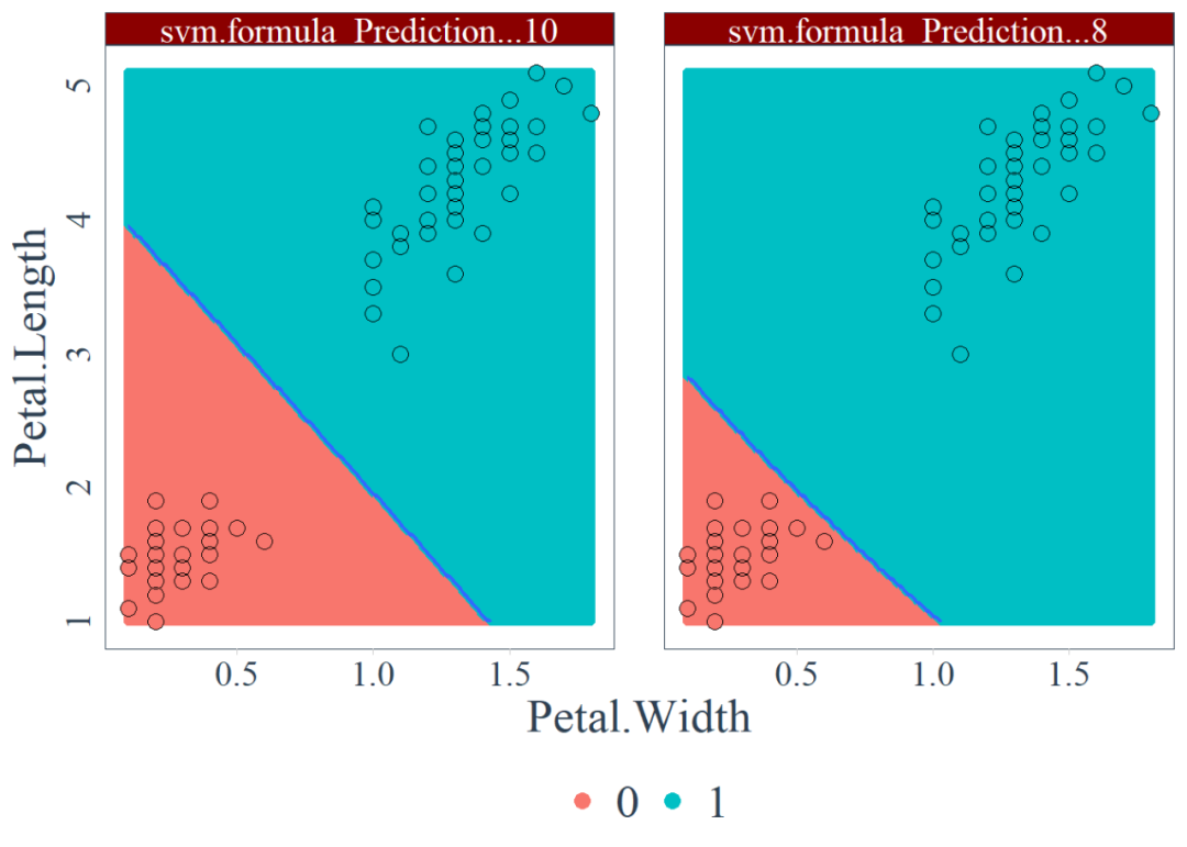
## $Petal.Width_and_Petal.Length
## $Petal.Length_and_Petal.Width## Warning in grDevices::contourLines(x = sort(unique(data$x)), y =## sort(unique(data$y)), : todos los valores de z son iguales## Warning: Not possible to generate contour data
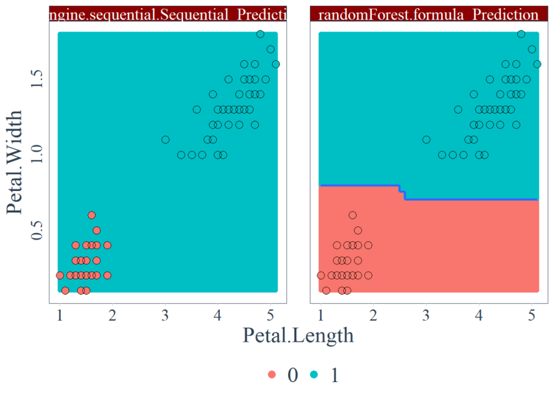
通常线性模型会产生线性的决策边界。看起来Random Forest模型会过拟合一些数据,而XGBoost和LightGBM模型能够得到更好且更通用的决策边界。Keras神经网络的性能较差,因为还没有训练到位。glm = 逻辑回归模型
svm.formula Prediction...6 = 支持向量机+线性核
svm.formula Prediction...8 = 支持向量机+多项式核
svm.formula Prediction...12 = 支持向量机 +径向核
svm.formula Prediction...10 = 支持向量机+sigmoid核
randomForest.formula Prediction =随机森林
xgb.Booster Prediction = 默认参数下的XGBoost模型
keras.engine.sequential.Sequential Prediction...18 = 单层Keras神经网络
keras.engine.sequential.Sequential Prediction...18 = 更深层的Keras神经网络
keras.engine.sequential.Sequential Prediction...22 = 更深一层的Keras神经网络
lgb.Booster Prediction = 默认参数下的LightGBM模型
在许多组合中,Keras神经网络模型只是预测所有观测值都属于某一类别(同样,我对模型没有进行很多调整,以及模型只有100个观测值来训练却要对40,000个点进行预测)。也就是说它将整个背景颜色染成蓝色或红色,并进行了许多错误分类。在某些图中,神经网络可以实现完美的分类,而在另一些图中则做出了奇怪的决策边界---神经网络很有趣。对这些图作一些简要分析,看起来我们用简单的逻辑回归模型得到了近乎完美的分类。但是由于每个变量的关系都是线性可分离的,这并不令人惊讶。但我仍偏爱XGBoost和LightGBM模型,因为它们可以通过在其目标函数中加入正则化来处理非线性关系,从而得到更可靠的决策边界。随机森林模型在这里失败了,他们的决策边界看起来做得很好,但其实也有些模糊和尖锐的部分。但当然,随着更多变量和更大维度的出现,这些决策边界会变得更加复杂和非线性。for(i in 1:length(plot_data)){ print(ggplot_lists[[i]]) }
我是在Amazon Ubuntu EC2实例上编写此模型的,但是,当我在Windows系统上用R编译博客文章时,遇到了一些问题。这些问题主要归因于安装lightgbm软件包和软件包版本。使用以下软件包版本(即使用最新的软件包版本),代码正常运行。sessionInfo()
## R version 3.6.1 (2019-07-05)## Platform: x86_64-w64-mingw32/x64 (64-bit)## Running under: Windows 10 x64 (build 17763)#### Matrix products: default#### locale:## [1] LC_COLLATE=Spanish_Spain.1252 LC_CTYPE=Spanish_Spain.1252 ## [3] LC_MONETARY=Spanish_Spain.1252 LC_NUMERIC=C ## [5] LC_TIME=Spanish_Spain.1252 ##
## attached base packages:## [1] stats graphics grDevices utils datasets methods base #### other attached packages:## [1] tidyquant_0.5.7 quantmod_0.4-15 ## [3] TTR_0.23-6 PerformanceAnalytics_1.5.3## [5] xts_0.11-2 zoo_1.8-6 ## [7] lubridate_1.7.4 keras_2.2.5.0 ## [9] lightgbm_2.3.2 R6_2.4.1 ## [11] xgboost_0.90.0.1 tidyr_1.0.0 ## [13] stringr_1.4.0 purrr_0.3.2 ## [15] kableExtra_1.1.0.9000 knitr_1.25.4 ## [17] ggplot2_3.2.1 patchwork_1.0.0 ## [19] dplyr_0.8.99.9000 #### loaded via a namespace (and not attached):## [1] Rcpp_1.0.3 lattice_0.20-38 class_7.3-15 ## [4] utf8_1.1.4 assertthat_0.2.1 zeallot_0.1.0 ## [7] digest_0.6.24 e1071_1.7-2 evaluate_0.14 ## [10] httr_1.4.1 blogdown_0.15 pillar_1.4.3.9000 ## [13] tfruns_1.4 rlang_0.4.4 lazyeval_0.2.2 ## [16] curl_4.0 rstudioapi_0.10 data.table_1.12.8 ## [19] whisker_0.3-2 Matrix_1.2-17 reticulate_1.14-9001## [22] rmarkdown_1.14 lobstr_1.1.1 labeling_0.3 ## [25] webshot_0.5.1 readr_1.3.1 munsell_0.5.0 ## [28] compiler_3.6.1 xfun_0.8 pkgconfig_2.0.3 ## [31] base64enc_0.1-3 tensorflow_2.0.0 htmltools_0.3.6 ## [34] tidyselect_1.0.0 tibble_2.99.99.9014 bookdown_0.13 ## [37] quadprog_1.5-7 randomForest_4.6-14 fansi_0.4.1 ## [40] viridisLite_0.3.0 crayon_1.3.4 withr_2.1.2 ## [43] rappdirs_0.3.1 grid_3.6.1 Quandl_2.10.0 ## [46] jsonlite_1.6.1 gtable_0.3.0 lifecycle_0.1.0 ## [49] magrittr_1.5 scales_1.0.0 rlist_0.4.6.1 ## [52] cli_2.0.1 stringi_1.4.3 xml2_1.2.2 ## [55] ellipsis_0.3.0 generics_0.0.2 vctrs_0.2.99.9005 ## [58] tools_3.6.1 glue_1.3.1 hms_0.5.1 ## [61] yaml_2.2.0 colorspace_1.4-1 rvest_0.3.4
Decision Boundary for a Series of Machine Learning Modelshttps://www.kdnuggets.com/2020/03/decision-boundary-series-machine-learning-models.html译者简介:张若楠,UIUC统计研究生毕业,南加州传媒行业data scientist。曾实习于国内外商业银行,互联网,零售行业以及食品公司,喜欢接触不同领域的数据分析与应用案例,对数据科学产品研发有很大热情。
END
转自: 数据派THU 公众号;
版权声明:本号内容部分来自互联网,转载请注明原文链接和作者,如有侵权或出处有误请和我们联系。
合作请加QQ:365242293
数据分析(ID : ecshujufenxi )互联网科技与数据圈自己的微信,也是WeMedia自媒体联盟成员之一,WeMedia联盟覆盖5000万人群。